Bayesian Inference

NYU Applied Statistics for Social Science Research

Eric Novik

Spring 2026 | Lecture 1

New York University

Introductions

• State your name and where you are from
• What is your field of study/work, and what are you hoping to learn in this class

\[ \DeclareMathOperator{\E}{\mathbb{E}} \DeclareMathOperator{\P}{\mathbb{P}} \DeclareMathOperator{\V}{\mathbb{V}} \DeclareMathOperator{\L}{\mathscr{L}} \DeclareMathOperator{\I}{\text{I}} \DeclareMathOperator{\d}{\mathrm{d}} \]

Lecture 1: Bayesian Workflow

• Overview of the course
• Subjective vs Objective
• Statistics vs AI/ML
• Brief history of Bayesian inference
• Stories: pricing books and developing drugs
• Review of probability and simulations
• Bayes’s rule
• Introduction to Bayesian workflow
• Wanna bet? Mystery box game

Subjective vs Objective

• An experienced sommelier is able to correctly identify 8 types of wine from 8 samples
• An astrologer was able to correctly predict if the stock market is up or down 8 times in a row
• Is your inference about their predictive ability different? The data are the same!
• Should we let data speak?

Statistics vs. AI/ML (Simplification!)

• AI is about automating tasks that humans are able to do
  • Recognizing faces, cats, and other objects
  • Identifying tumors on a radiology scan
  • Playing Chess and Go
  • Driving a car
  • Post ChatGPT 4: Generating coherent text/images/video, signs of reasoning

• Statistics is useful for answering questions that humans are not able to do
  • How fast does a drug clear from the body?
  • What is the expected tumor size two months after treatment?
  • How would patients respond under a different treatment?
  • Should I take this drug?
  • Should we (FDA/EMA/…) approve this drug?

Note

“Machine learning excels when you have lots of training data that can be reasonably modeled as exchangeable with your test data; Bayesian inference excels when your data are sparse and your model is dense.” — Andrew Gelman

Turn to your neighbor and discuss

Classify each of the following: {decision, parameter inference, prediction, causal inference}

1. How fast does a drug clear from the body?
2. What is the expected tumor size two months after treatment?
3. How would patients respond under a different treatment?
4. Should I take this drug?
5. Should we (FDA/EMA/…) approve this drug?

Question

Which category is missing data imputation?

Brief History

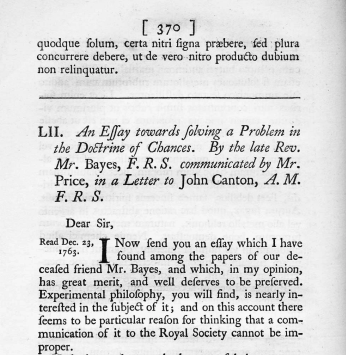
Summary of the book The Theory That Would Not Die

• Thomas Bayes (1702(?) — 1761) is credited with the discovery of the “Bayes’s Rule”
• His paper was published posthumously by Richard Price in 1763
• Laplace (1749 — 1827) independently discovered the rule and published it in 1774
• Scientific context: Newton’s Principia was published in 1687
• Bayesian wins: German Enigma cipher, search for a missing H-bomb, Federalist papers, Moneyball, FiveThirtyEight

Stephen Stigler gives 3:1 in favor of Nicholas Saunderson for the discovery of Bayes’s [sic] rule.

Laplace’s Demon

We may regard the present state of the universe as the effect of its past and the cause of its future. An intellect which at any given moment knew all of the forces that animate nature and the mutual positions of the beings that compose it, if this intellect were vast enough to submit the data to analysis, could condense into a single formula the movement of the greatest bodies of the universe and that of the lightest atom; for such an intellect nothing could be uncertain, and the future just like the past would be present before its eyes.

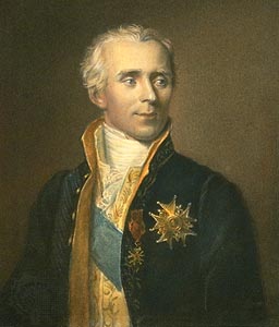
Marquis Pierre Simon de Laplace (1749 — 1827)

“Uncertainty is a function of our ignorance, not a property of the world.”

Modern Examples of Bayesian Analyses

Elasticity of Demand

Stan with Hierarchical Models

Pharmacokinetics of Drugs

Stan with Ordinary Differential Equations

Nonparametric Bayes

Stan with Gaussian Processes

Example Simulation

• We will use R’s sample() function to simulate rolls of a die and replicate() function to repeat the rolling process many times

die <- 1:6; N <- 1e4
roll <- function(x, n) {
  sample(x, size = n, replace = TRUE)
}
roll(die, 2) # roll the die twice

[1] 5 3

rolls <- replicate(N, roll(die, 2))
rownames(rolls) <- c("X1", "X2")
rolls[, 1:10] # print first 10 outcomes

   [,1] [,2] [,3] [,4] [,5] [,6] [,7] [,8] [,9] [,10]
X1    6    4    3    2    2    5    1    4    5     4
X2    3    4    4    5    1    1    6    6    6     5

Y <- colSums(rolls) # Y = X1 + X2
head(Y)

[1] 9 8 7 7 3 6

mean(Y < 11) # == 1/N * sum(Y < 11)

[1] 0.9137

• Given a Random Variable \(Y\), \(y^{(1)}, y^{(2)}, y^{(3)}, \ldots, y^N\) are simulations or draws from \(Y\)
• Fundamental bridge (Blitzstein & Hwang p. 164): \(\P(A) = \E(\I_A)\)
• For \(Y = X_1 + X_2\): \(\P(Y < 11) \approx \frac{1}{N} \sum^{N}_{n=1} \I(y^n < 11)\)
• In R, \(Y < 11\) creates an indicator variable
• And mean() does the average

Example Simulation

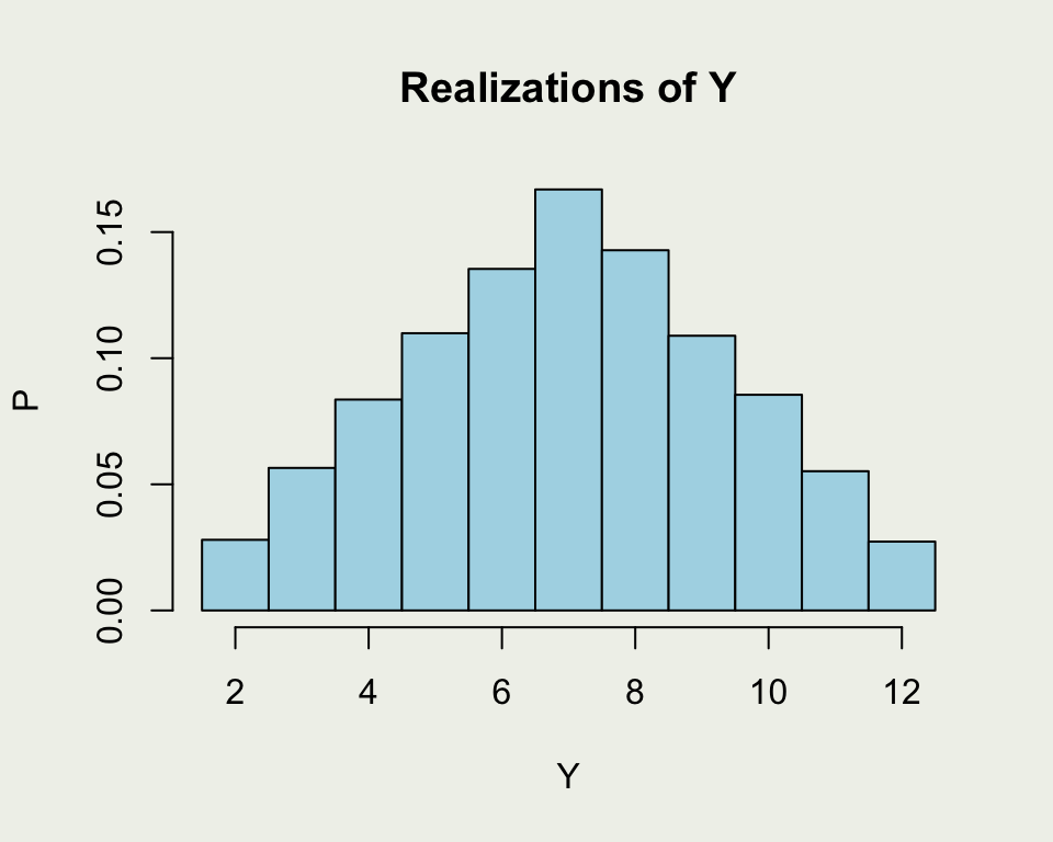
This is a more direct demonstration of random draws from a distribution of \(Y = X_1 + X_2\)

# Define the possible values of 
# Y = X1 + X2 and their probabilities

Omega <- 2:12
Y_probs <- 
  c(1, 2, 3, 4, 5, 6, 5, 4, 3, 2, 1) / 36

# Simulate 10,000 realizations of Y
Y_samples <- sample(Omega,
                    size = 1e4, 
                    replace = TRUE, 
                    prob = Y_probs)

# Compute Pr(A)
mean(Y_samples < 11)

[1] 0.9175

# Plot a histogram of the realizations of Y
par(bg = "#f0f1eb")
hist(Y_samples, 
     breaks = seq(1.5, 12.5, by = 1), 
     main = "Realizations of Y",
     xlab = "Y", ylab = "P",
     col = "lightblue",
     prob = TRUE)

Can’t Stop Board Game

Law of Total Probability (LOTP)

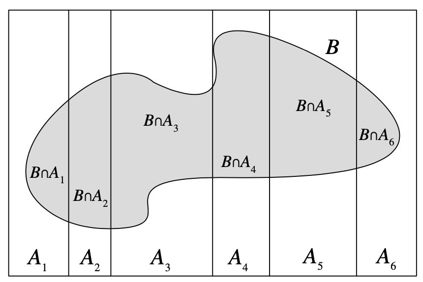
Let \(A\) be a partition of \(\Omega\), so that each \(A_i\) is disjoint, \(\P(A_i >0)\), and \(\cup A_i = \Omega\). \[ \P(B) = \sum_{i=1}^{n} \P(B \cap A_i) = \sum_{i=1}^{n} \P(B \mid A_i) \P(A_i) \]

BIPEPSE: AI as a tutor

Suppose you forgot the law of iterated expectations (Adam’s Law) which states \[ \E(Y) = \E_X(\E_{Y|X}(Y \mid X)) \]

Use the following AI prompts

• Background: I am a Masters student in Statistics. I want to go over the law of iterated expectations. Intuition: First, give me an intuitive explanation. I will ask a follow-up question after.
• Proof: Please, provide a step-by-step proof of the discrete case, explaining every move.
• Example: Please provide a numerical example.
• Problem: Now, please give me a practice problem.
• Simulation: Write a simulation and ask AI to check it OR say: write a simulation in R
• Explanation: How is this for an explanation? [Enter an explanation in your words and have it check you]

Adam’s Law Simulation

library(purrr)
n <- 20
class_sizes <- sample(n)
mean_gpa_vec <- runif(n = n, 2.8, 3.2)
N <- sum(class_sizes)
W <- class_sizes / N
G <- class_sizes |>
  map(\(x) rnorm(n = x, mean = mean_gpa_vec, sd = 1))

# E(Y)
EY <- unlist(G) |> mean()
print(EY)

# E(E(Y | X))
class_means <- map_dbl(G, mean) # can't just average those
gpaXprob <- class_means * W
EEYX <- sum(gpaXprob)
print(EEYX)

Bivariate Case

• A bivariate CDF \(F_{X,Y}(x, y) = \P(X \leq x, Y \leq y)\)

\[ F_{X,Y}(x, y) \geq 0 \quad \text{for all } x, y \]

• If the PDF exists

\[ F_{X,Y}(x, y) = \int_{-\infty}^x \int_{-\infty}^y f_{X,Y}(u, v) \, \mathrm{d}v \, \mathrm{d}u \]

• Normalization

\[ \int_{-\infty}^\infty \int_{-\infty}^\infty f_{X,Y}(x, y) \, \mathrm{d}x \, \mathrm{d}y = 1 \]

• From CDF to PDF

\[ f_{X,Y}(x, y) = \frac{\partial^2}{\partial x \partial y} F_{X,Y}(x, y) \]

Bivariate Case

• Marginalization

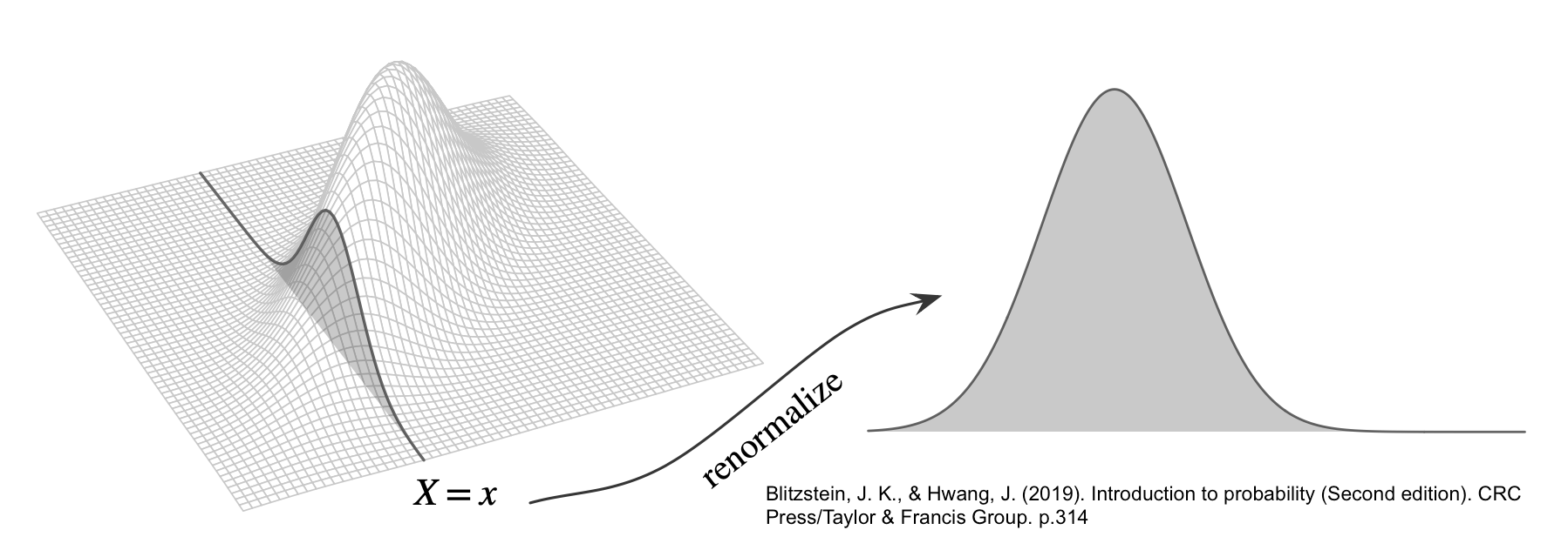
\[ f_Y(y) = \int_{-\infty}^\infty f_{X,Y}(x, y) \, \mathrm{d}x. \]

• Conditional CDF

\[ F_{Y \mid X}(y \mid x) = \P(Y \leq y \mid X = x) \]

• Conditional PDF: a function of \(y\) for fixed \(x\) \[ f_{Y|X}(y \mid x) = \frac{f_{X,Y}(x, y)}{f_X(x)} \]

Bivariate Normal

\[ f_{X,Y}(x, y) = \frac{1}{2 \pi \sqrt{\det(\Sigma)}} \exp\left( -\frac{1}{2} \begin{bmatrix} x - \mu_X \\ y - \mu_Y \end{bmatrix}^\top \Sigma^{-1} \begin{bmatrix} x - \mu_X \\ y - \mu_Y \end{bmatrix} \right) \]

\[ \Sigma = \begin{bmatrix} \sigma_X^2 & \rho\,\sigma_X\sigma_Y \\ \rho\,\sigma_X\sigma_Y & \sigma_Y^2 \end{bmatrix}, \quad \rho = \frac{\operatorname{Cov}(X, Y)}{\sigma_X \, \sigma_Y}, \quad -1 \leq \rho \leq 1 \]

Bivariate Normal Demo

library(distributional)

sigma_X <- 1
sigma_Y <- 2
rho <- 0.3  # Correlation coefficient

rho_sigmaXY <- rho * sigma_X * sigma_Y # why?

cov_matrix <- matrix(c(sigma_X^2,   rho_sigmaXY,
                       rho_sigmaXY, sigma_Y^2), 2, 2)

dmv_norm <- dist_multivariate_normal(mu    = list(c(0, 0)), 
                                     sigma = list(cov_matrix))
dimnames(dmv_norm) <- c("x", "y")
variance(dmv_norm)

     x y
[1,] 1 4

covariance(dmv_norm)

[[1]]
       x   y
[1,] 1.0 0.6
[2,] 0.6 4.0

density(dmv_norm, cbind(3, 3)) |> round(2)   # should be low

[1] 0

cdf(dmv_norm, cbind(3, 3)) |> round(2)       # should be high

[1] 0.93

Bivariate Normal Demo: Sampling

# draws from the bivariate normal
draws <- generate(dmv_norm, 1e4)            
str(draws)

List of 1
 $ : num [1:10000, 1:2] 1.9664 0.0325 1.785 0.1801 0.0296 ...
  ..- attr(*, "dimnames")=List of 2
  .. ..$ : NULL
  .. ..$ : chr [1:2] "x" "y"

draws <- as_tibble(draws[[1]])
head(draws)

# A tibble: 6 × 2
       x      y
   <dbl>  <dbl>
1 1.97   -1.40 
2 0.0325  1.63 
3 1.79    1.15 
4 0.180  -0.554
5 0.0296  3.58 
6 0.0433  0.243

# estimated means
colMeans(draws) |> round(2)

    x     y 
-0.01  0.00 

# estimated covariance matrix
cov(draws) |> round(2)

     x    y
x 0.98 0.60
y 0.60 3.97

# estimated correlations matrix
cor(draws) |> round(2)

    x   y
x 1.0 0.3
y 0.3 1.0

# should be close to cdf(dist, cbind(3, 3)); why?
# both evaluate to P(X and Y < 3)
# & is an _and_ operator
mean(draws$x < 3 & draws$y < 3) |> round(2)

[1] 0.93

# P(X < 0 or Y < 1)
# | is an _or_, not conditioning operator
mean(draws$x < 0 | draws$y < 1) |> round(2)

[1] 0.8

Bivariate Normal Demo: Analytical

How would we do the above analytically? \[ \P(X < 0 \cup Y < 1) = \P(X < 0) + \P(Y < 1) - \P(X < 0 \cap Y < 1) \]

# Compute P(X < 0)
p_X_less_0 <- cdf(dist_normal(mu = 0, sigma = sigma_X), 0) # pnorm(0, mean = 0, sd = sigma_X)

# Compute P(Y < 1)
p_Y_less_1 <- cdf(dist_normal(mu = 0, sigma = sigma_Y), 1) # pnorm(1, mean = 0, sd = sigma_Y)

# Compute P(X < 0, Y < 1)
p_X_less_0_and_Y_less_1 <- cdf(dmv_norm, cbind(0, 1))

# P(X < 0 or Y < 1)
(p_X_less_0 + p_Y_less_1 - p_X_less_0_and_Y_less_1) |> round(2)

[1] 0.8

• Would you rather do mean(draws$x < 0 | draws$y < 1) or the analytical solution?
• How would you evaluate \(\P(X < 0 \mid Y < 1)\)

draws |> filter(y < 1) |>
  summarise(pr = mean(x < 0)) |>
  as.numeric() |> round(2)

[1] 0.56

Bayes’s Rule

• Bayes’s rule for events

\[ \P(A \mid B) = \frac{\P(A \cap B)}{\P(B)} = \frac{\P(B \mid A) \P(A)}{\sum_{i=1}^{n} \P(B \mid A_i) \P(A_i)} \]

• Bayes’s rule for continuous RVs

\[ \underbrace{\color{blue}{f_{\Theta|Y}(\theta \mid y)}}_{\text{Posterior}} = \frac{ \overbrace{ \color{red}{f_{Y|\Theta}(y \mid \theta)} }^{\text{Likelihood}} \cdot \overbrace{\color{green}{f_\Theta(\theta)}}^{ \text{Prior} } }{ \underbrace{\int_{-\infty}^{\infty} f_{Y|\Theta}(y \mid \theta) f_\Theta(\theta) \, \text{d}\theta}_{\text{Prior Predictive } f(y)} } \propto \color{red}{f_{Y|\Theta}(y \mid \theta)} \cdot \color{green}{f_\Theta(\theta)} \]

Notation

• \(\theta\): unknowns or parameters to be estimated; could be multivariate, discrete, and continuous; in your book \(\pi\)
• \(y\): observations or measurements to be modelled (\(y_1, y_2, ...\))
• \(\widetilde{y}\) : unobserved but observable quantities; in your book \(y'\)
• \(x\): covariates
• \(f( \theta )\): a prior model, P[DM]F of \(\theta\)
• \(f(y \mid \theta, x)\): an observational model, P[DM]F when it is a function of \(y\); in your book: \(f(y \mid \pi)\)
• \(f(y \mid \theta)\): is a likelihood function when it is a function of \(\theta\); in your book: \(\L(\pi \mid y)\)
• Some people write \(\L(\theta; y)\) or simply \(\L(\theta)\)
• \(U(z)\): utility function where \(z\) can be some \(g(\theta, \tilde{y})\)
• \(\E(U(z) \mid d)\): expected utility for decision \(d\)

Bayesian Workflow in a Nutshell

• Specify a prior model \(f(\theta)\)
• Pick a data model \(f(y \mid \theta, x)\), including conditional mean: \(\E(y \mid x)\)
• Set up a prior predictive distribution \(f(y)\)
• After observing data \(y\), we treat \(f(y \mid \theta, x)\) as the likelihood of observing \(y\) under all plausible values of \(\theta\), conditioning on \(x\) if necessary
• Derive a posterior distribution for \(\theta\), \(\, f(\theta \mid y, x)\)
• Evaluate model quality: 1) quality of the inferences; 2) quality of predictions; go back to the beginning
• Compute derived quantities, such as \(\P(\theta > \alpha)\), \(f(\widetilde{y} \mid y)\), and \(d^* = \textrm{arg max}_d \ \E(U(z) \mid d)\)

Mystery Box Game Analysis

• You are invited to bet on the proportion of red balls
• True proportions: \(\theta \in \{0.25,\, 0.50,\, 0.75\}\)
• You are allowed to draw 5 balls from the box with replacement and wager $5
• Net payoffs (Gross payoffs - your wager) if your chosen \(\theta\) is correct:
  • For \(\theta=0.25\): $5
  • For \(\theta=0.50\): $10
  • For \(\theta=0.75\): $25
• Does it make sense to assume that each box type is equally likely?
• Work out the implied probabilities based on the payoffs, assuming fair game
• Go to https://ericnovik.github.io/apps/, click on Mystery Box and play 20 rounds

Game and Prior

• Select one box at random
• Draw 5 balls from the box
• You can pay $5 and play (make a guess), or pay $0.50 for extra ball and play
• If you buy an extra ball, you pay $5 and play
• For warm-ups: you select a box and draw one ball – what is \(\P(\text{red})\)?
• Law of Total Probability (LOTP):

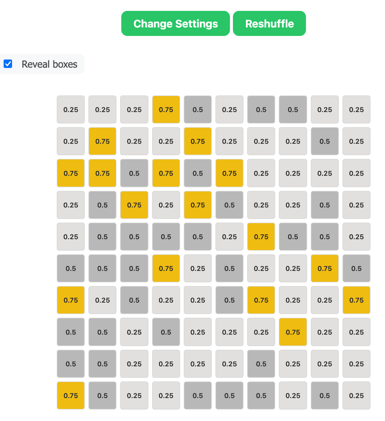
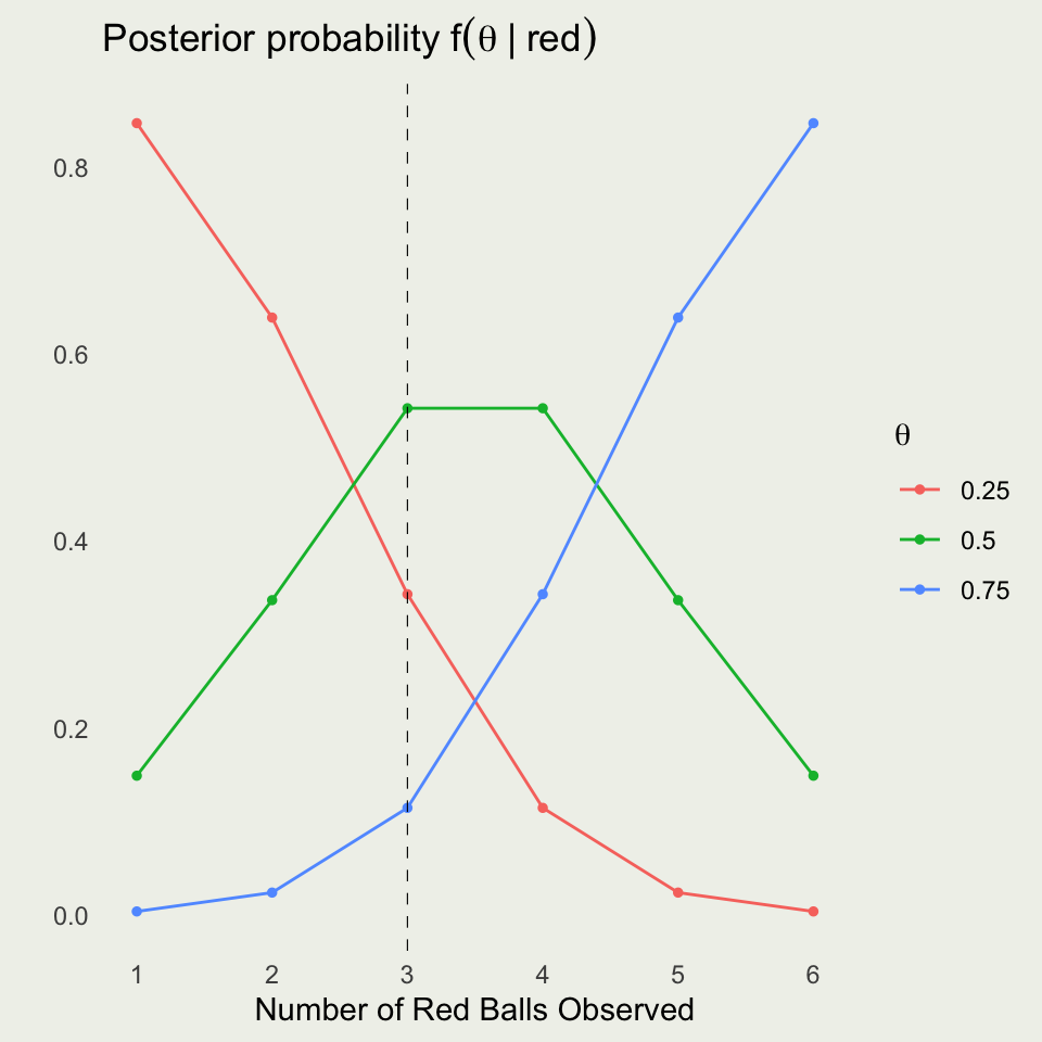
\[ \begin{eqnarray*} \P(\text{red}) &=& \sum_{i=1}^{3} f(\text{red},\ \theta_i) = \sum_{i=1}^{3} f(\text{red} \mid \theta_i) \cdot f(\theta_i) \\ &=& 0.25 \cdot \left(\frac{1}{2}\right) + 0.50 \cdot \left(\frac{1}{3}\right) + 0.75 \cdot \left(\frac{1}{6}\right) \approx 0.42 \end{eqnarray*} \]

Data Model: Before Drawing 5 Balls

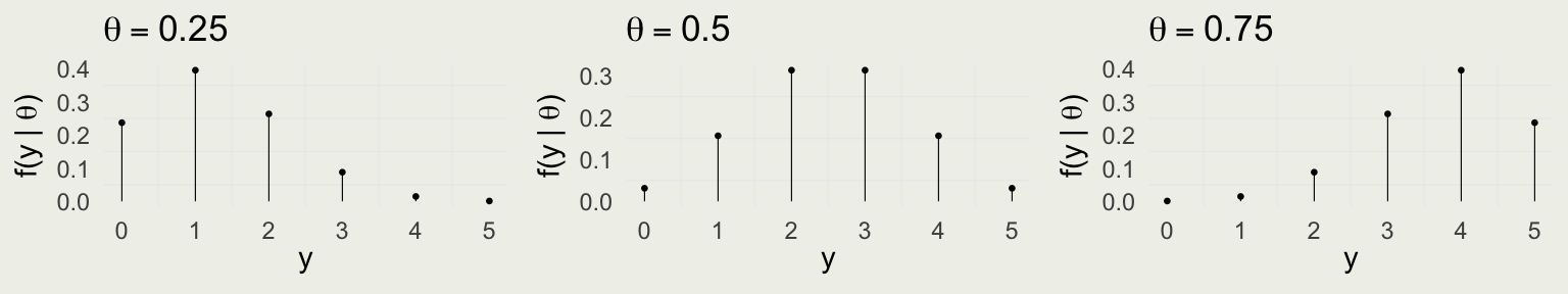
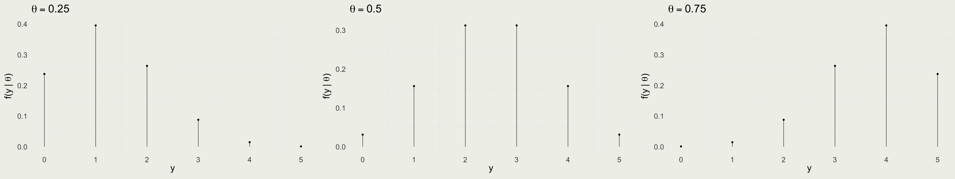
• Take red ball as success, so \(y\) successes out of \(N = 5\) trials \[ y | \theta \sim \text{Bin}(N,\theta) = \text{Bin}(5,\theta) \]

• \(f(y \mid \theta) = \text{Bin} (y \mid 5,\theta) = \binom{5}{y} \theta^y (1 - \theta)^{5 - y}\) for \(y \in \{0,1,\ldots,5\}\)

• Is this a valid probability distribution as a function of \(y\)?

N = 5; y <- 0:N
f_y <- dbinom(x = y, size = N, prob = theta[1])
sum(f_y)

[1] 1

Likelihood Function: After Drawing 5 Balls

• We observe that 2 out of 5 balls are red
• We can construct a likelihood function for \(y = 2\) as a function of \(\theta\)

\[ f(\theta \mid y = 2) = \binom{5}{2} \theta^2 (1 - \theta)^{3} \]

• This is a function of \(\theta\), not \(y\)
• Is the likelihood a probability distribution? It does not integrate to 1 over \(\theta\):

dbinom_theta <- function(theta, N, y) {
  choose(N, y) * theta^y * (1 - theta)^(N - y)
}
integrate(dbinom_theta, lower = 0, upper = 1,
          N = 5, y = 2)[[1]] |> fractions()

[1] 1/6

Prior Predictive Distribution

• The integral of the likelihood over \(\theta\) (under a uniform prior) gives us the prior predictive distribution: \[ f(y) = \int_{0}^{1} \binom{N}{y} \theta^y (1 - \theta)^{N - y}\, d\theta = \frac{1}{N + 1} \]
• \(f(y)\) is called the marginal distribution or prior predictive distribution
• It tells us that prior to observing \(y\), all values of \(y\) are equally likely

Visualizing the Likelihood Function

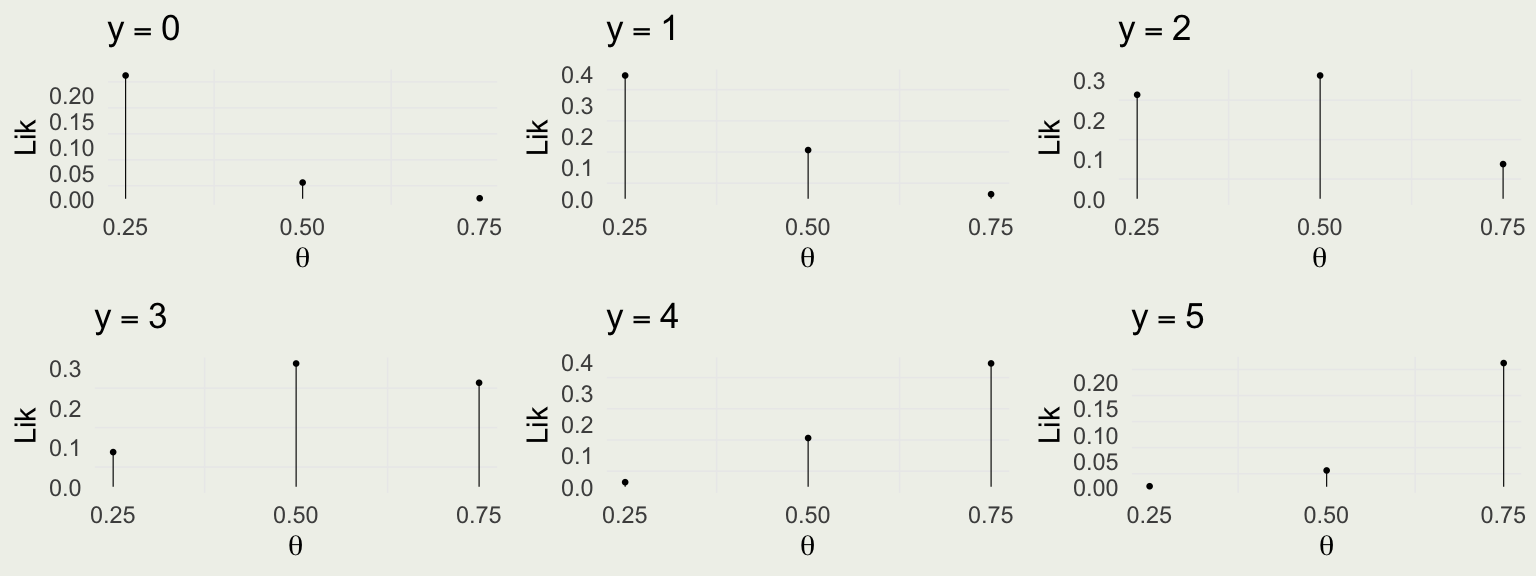
Compare with the data model:

Putting It All Together

• We observe 2 red balls, so we can condition on \(y = 2\)
• Let’s turn the Bayesian crank

\[ \begin{eqnarray*} f(\theta \mid y) &=& \frac{f(y \mid \theta) f(\theta)}{f(y)} = \frac{f(y \mid \theta) f(\theta)}{\sum_{i=1}^{3} f(y, \, \theta_i)} = \frac{f(y \mid \theta) f(\theta)}{\sum_{i=1}^{3} f(y \mid \theta_i) f(\theta_i)} \\ &\propto& f(y \mid \theta) f(\theta) \propto \theta^2 (1 - \theta)^{3} \cdot f(\theta) \end{eqnarray*} \]

• How many elements in \(f(\theta)\)?
• How many elements in \(f(\theta \mid y)\)?

Compute the Posterior

• We observed \(y = 2\), so \(f(y \mid \theta) \propto \theta^2 (1 - \theta)^{3}\)

• For \(\theta = 0.25\): (we can drop \(\binom{5}{2}\) term) \[ f(y | 0.25) = \binom{5}{2} (0.25)^2 (0.75)^3 \approx 0.26 \]
• For \(\theta = 0.50\): \[ f(y | 0.50) = \binom{5}{2} (0.50)^5 \approx 0.31 \]
• For \(\theta = 0.75\): \[ f(y| 0.75 ) = \binom{5}{2} (0.75)^2 (0.25)^3 \approx 0.09 \]

N <- 5; y <- 2
theta <- c(0.25, 0.50, 0.75)
prior <- c(1/2, 1/3, 1/6)
lik <- dbinom(y, N, theta)
lik_x_prior <-  lik * prior
norm_const <- sum(lik_x_prior)
post <- lik_x_prior / norm_const

theta	prior	lik	lxp	post
0.25	0.50	0.26	0.13	0.53
0.5	0.33	0.31	0.10	0.42
0.75	0.17	0.09	0.01	0.06
Total	1.00	0.66	0.25	1.00

Option 1: Play Immediately

• Let \(x_i\) represent the gross payoffs for each option \(i\) (\(10, 15, 30\))
• We maximize Expected Utility:

\[ \theta^* = \textrm{arg max}_{\theta} \left\{ x_i \times f(\theta_i \mid y) - \text{Cost} \right\} \]

• Bet on \(\theta=0.25\): \(10 \times 0.526 - 5 \approx \$0.26\)
• Bet on \(\theta=0.50\): \(15 \times 0.416 - 5 \approx \$1.24\)
• Bet on \(\theta=0.75\): \(30 \times 0.058 - 5 \approx -\$3.26\)
• We bet on \(\theta^*=0.50\) with expected payoff of $1.24.

The Conflict

The bet on the most probable outcome (MAP estimate of \(\theta=0.25\) at 53%) is suboptimal!

Because of the asymmetric payoffs, we bet on \(\theta=0.50\) despite it having a lower posterior probability (42%).

Option 2: Should You Buy an Extra Ball?

• We need to average over uncertainty of the red vs green ball
• We use the current posterior weights \(f(\theta \mid y)\), where y is 2 reds out of 5
• Compute the probability of red on the next draw (Posterior Predictive Distribution):

\[ \begin{eqnarray*} f(\text{red} \mid y) &=& \sum_{i=1}^{3} f(\text{red}, \ \theta_i \mid y) = \sum_{i=1}^{3} f(\text{red} \mid \theta_i, \ y) f(\theta_i \mid y) \\ &=& \sum_{i=1}^{3} f(\text{red} \mid \theta_i) f(\theta_i \mid y) \\ f(\text{red} \mid y) &=& 0.25 \times 0.526 + 0.50 \times 0.416 + 0.75 \times 0.058 \\ &\approx& 0.383 \end{eqnarray*} \]

• Posterior predictive probability of green: \(f(\text{green} \mid y) = 1 - 0.383 \approx 0.617\)

Updating Beliefs: Case 1 — Extra Ball is Red

If the extra ball is red, we update our posterior using Bayes’s rule, treating \(f(\theta_i \mid y)\) as the prior:

\[ f(\theta_i \mid y, \text{red}) = \frac{f(\text{red} \mid \theta_i, y) \cdot f(\theta_i \mid y)}{f(\text{red} \mid y)} \]

• Since draws are independent given \(\theta\): \(\,f(\text{red} \mid \theta_i, y) = f(\text{red} \mid \theta_i) = \theta_i\)
• Expand the denominator via LOTP: \(\,f(\text{red} \mid y) = \sum_{j=1}^{3} \theta_j \cdot f(\theta_j \mid y) = 0.383\)

\[ f(\theta_i \mid y, \text{red}) = \frac{\overbrace{\theta_i}^{\text{Lik of red}} \cdot \overbrace{f(\theta_i \mid y)}^{\text{Current posterior}}} {\underbrace{\sum_{j=1}^{3} \theta_j \cdot f(\theta_j | y)}_{f(\text{red}|y) = 0.383}} \]

Exercise: Case 1 — Extra Ball is Red

Current posterior and gross payoffs:

\(\theta_i\)	\(f(\theta_i \mid y)\)	Gross payoff
0.25	0.526	$10
0.50	0.416	$15
0.75	0.058	$30

\[ \text{Prize}_i = \text{payoff}_i \times f(\theta_i \mid y, \text{red}) \]

Which \(\theta\) should you bet on if the next ball is red?

Updating Beliefs: Case 1 — Solution

• Unnormalized weights \(\theta_i \cdot f(\theta_i \mid y)\):
  • For \(\theta=0.25\): \(0.526 \times 0.25 = 0.1315\)
  • For \(\theta=0.50\): \(0.416 \times 0.50 = 0.2080\)
  • For \(\theta=0.75\): \(0.058 \times 0.75 = 0.0435\)
• Normalized probabilities (divide by \(0.1315 + 0.2080 + 0.0435 = 0.383\)):
  • \(f(0.25 \mid y,\, \text{red}) \approx 0.343\), \(\quad f(0.50 \mid y,\, \text{red}) \approx 0.543\), \(\quad f(0.75 \mid y,\, \text{red}) \approx 0.114\)
• Expected gross prizes:
  • Bet on \(\theta=0.25\): \(0.343 \times 10 \approx 3.43\)
  • Bet on \(\theta=0.50\): \(0.543 \times 15 \approx \mathbf{8.15}\)
  • Bet on \(\theta=0.75\): \(0.114 \times 30 \approx 3.42\)

Updating Beliefs: Case 2 — Extra Ball is Green

By the same logic, with \((1 - \theta_i)\) as the likelihood of green:

\[ f(\theta_i \mid y, \text{green}) = \frac{f(\text{green} \mid \theta_i) \cdot f(\theta_i \mid y)}{f(\text{green} \mid y)} = \frac{\overbrace{(1 - \theta_i)}^{\text{Lik of green}} \cdot \overbrace{f(\theta_i \mid y)}^{\text{Current posterior}}} {\underbrace{\sum_{j=1}^{3} (1 - \theta_j) \cdot f(\theta_j | y)}_{f(\text{green}|y) = 0.617}} \]

Exercise: Case 2 — Extra Ball is Green

Current posterior and gross payoffs:

\(\theta_i\)	\(f(\theta_i \mid y)\)	Gross payoff
0.25	0.526	$10
0.50	0.416	$15
0.75	0.058	$30

\[ \text{Prize}_i = \text{payoff}_i \times f(\theta_i \mid y, \text{green}) \]

Which \(\theta\) should you bet on if the next ball is green?

Updating Beliefs: Case 2 — Solution

• Unnormalized weights \((1 - \theta_i) \cdot f(\theta_i \mid y)\):
  • For \(\theta=0.25\): \(0.526 \times 0.75 = 0.3945\)
  • For \(\theta=0.50\): \(0.416 \times 0.50 = 0.2080\)
  • For \(\theta=0.75\): \(0.058 \times 0.25 = 0.0145\)
• Normalized probabilities (divide by \(0.3945 + 0.2080 + 0.0145 = 0.617\)):
  • \(f(0.25 \mid y,\, \text{green}) \approx 0.639\), \(\quad f(0.50 \mid y,\, \text{green}) \approx 0.337\), \(\quad f(0.75 \mid y,\, \text{green}) \approx 0.024\)
• Expected gross prizes:
  • Bet on \(\theta=0.25\): \(0.639 \times 10 \approx \mathbf{6.39}\)
  • Bet on \(\theta=0.50\): \(0.337 \times 15 \approx 5.06\)
  • Bet on \(\theta=0.75\): \(0.024 \times 30 \approx 0.72\)

Overall Expected Prize With the Extra Ball

• Combine the two cases:

  \[ \begin{align*} \E_\text{extra ball}({\text{payoff}}) =& f(\text{red} \mid y)\times 8.15 + f(\text{green} \mid y)\times 6.39 \\ =& 0.383 \times 8.15 + 0.617 \times 6.39 \approx 7.06 \end{align*} \]

• Net Expected Payoff (including costs):

  • Extra ball cost: $0.50
  • Play cost: $5

  \[ \E_\text{extra ball}({\text{payoff}}) = 7.06 - 5.50 = \$1.56. \]

• Without the extra ball: Net EV \(\approx \$1.24\).

• With the extra ball: Net EV \(\approx \$1.56\).

Decision: It is better to buy an extra ball for $0.50 before playing.

What About For All Possible Outcomes?

Net Payoffs With and Without Extra Ball?