     [,1] [,2] [,3] [,4] [,5] [,6]
[1,]    2    3    4    5    6    7
[2,]    3    4    5    6    7    8
[3,]    4    5    6    7    8    9
[4,]    5    6    7    8    9   10
[5,]    6    7    8    9   10   11
[6,] 7 8 9 10 11 12Bayesian Inference
NYU Applied Statistics for Social Science Research
Introductions
- State your name
- What is your field of study/work, and what are you hoping to learn in this class
- Go to: https://tinyurl.com/nyu-colab and write down where you are from (Country, City)

\[ \DeclareMathOperator{\E}{\mathbb{E}} \DeclareMathOperator{\P}{\mathbb{P}} \DeclareMathOperator{\V}{\mathbb{V}} \DeclareMathOperator{\L}{\mathscr{L}} \DeclareMathOperator{\I}{\text{I}} \DeclareMathOperator{\d}{\mathrm{d}} \]
Lecture 1: Bayesian Workflow
- Overview of the course
- Class participation: prediction intervals
- Statistics vs AI/ML
- Brief history of Bayesian inference
- Stories: pricing books and developing drugs
- Review of probability and simulations
- Bayes’s rule
- Introduction to Bayesian workflow
- Wanna bet? Mystery box game

Turn to your neighbor and discuss
Classify each of the following: {decision, parameter inference, prediction, causal inference}
- How fast does a drug clear from the body?
- What is the expected tumor size two months after treatment?
- How would patients respond under a different treatment?
- Should I take this drug?
- Should we (FDA/EMA/…) approve this drug?

Question
Which category is missing data imputation?
Brief History
Summary of the book The Theory That Would Not Die
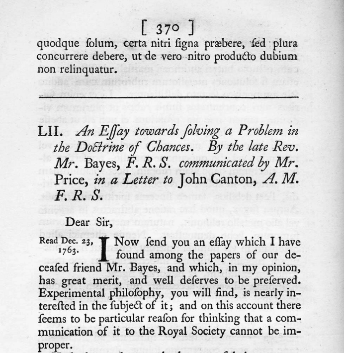
- Thomas Bayes (1702(?) — 1761) is credited with the discovery of the “Bayes’s Rule”
- His paper was published posthumously by Richard Price in 1763
- Laplace (1749 — 1827) independently discovered the rule and published it in 1774
- Scientific context: Newton’s Principia was published in 1687
- Bayesian wins: German Enigma cipher, search for a missing H-bomb, Federalist papers, Moneyball, FiveThirtyEight
Laplace’s Demon
We may regard the present state of the universe as the effect of its past and the cause of its future. An intellect which at any given moment knew all of the forces that animate nature and the mutual positions of the beings that compose it, if this intellect were vast enough to submit the data to analysis, could condense into a single formula the movement of the greatest bodies of the universe and that of the lightest atom; for such an intellect nothing could be uncertain, and the future just like the past would be present before its eyes.
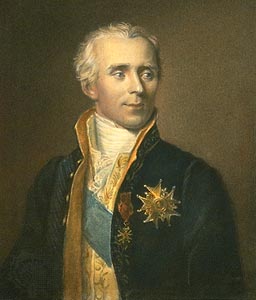
Marquis Pierre Simon de Laplace (1729 — 1827)
“Uncertainty is a function of our ignorance, not a property of the world.”
Modern Examples of Bayesian Analyses

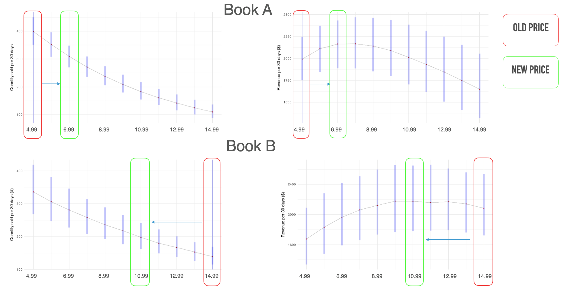
Elasticity of Demand
Stan with Hierarchical Models
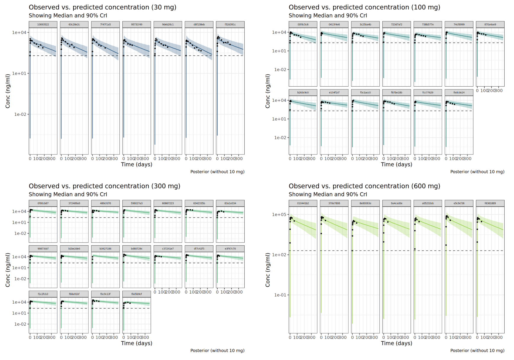
Pharmacokinetics of Drugs
Stan with Ordinary Differential Equations
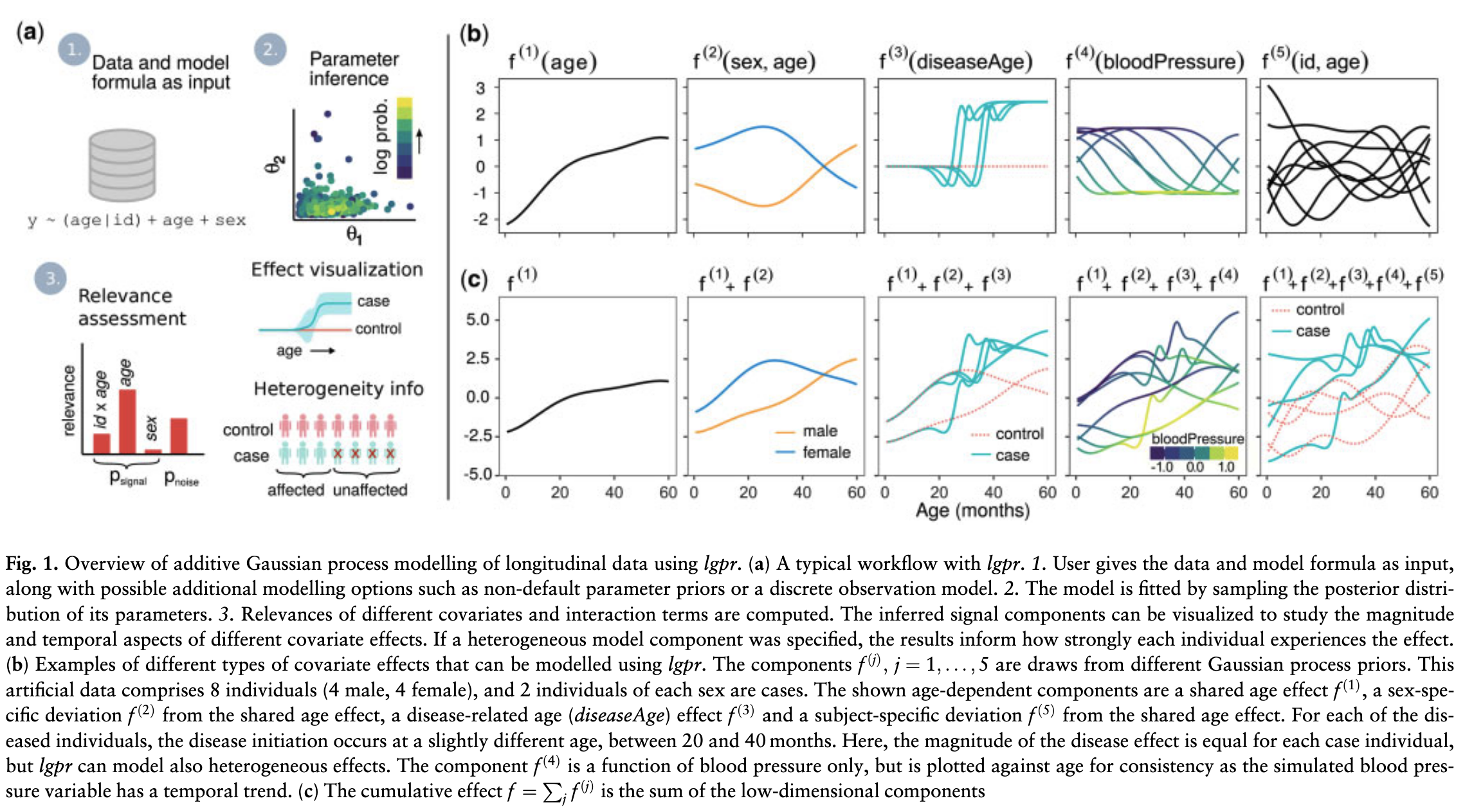
Nonparametric Bayes
Stan with Gaussian Processes
Random Variables Review
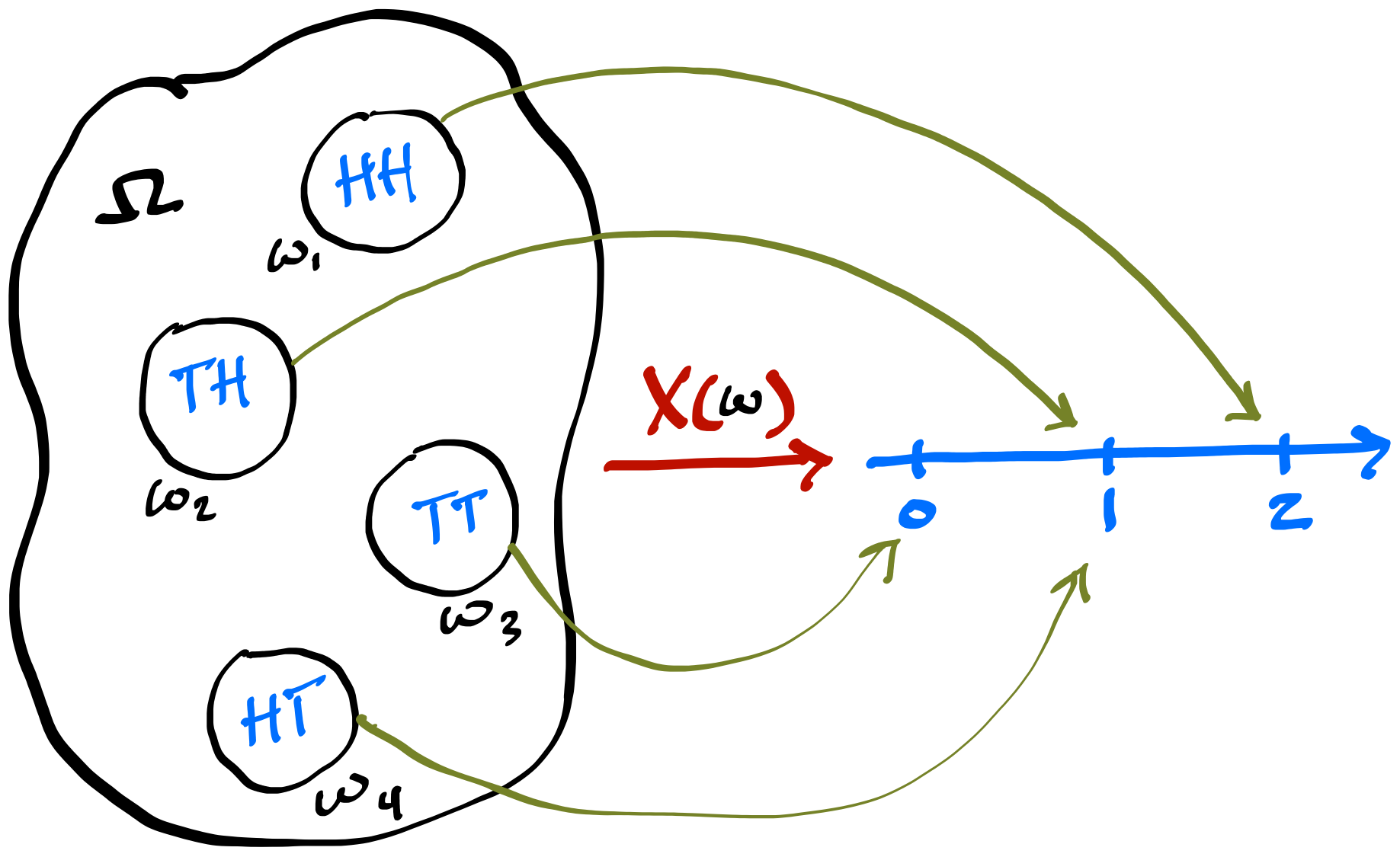
- A random variable \(X\) is a function that maps outcomes of a random experiment to real numbers. \(X: \Omega \to \mathbb{R}\). For each \(\omega \in \Omega\), \(X(\omega) \in\mathbb{R}\).
\[ \P_X(X = x_i) = \P\left(\{\omega_j \in \Omega : X(\omega_j) = x_i\}\right) \]
- PMF, PDF, CDF (Blitzstein and Hwang, Ch. 3, 5)
- Expectations (Blitzstein and Hwang, Ch. 4)
- Joint Distributions (Blitzstein and Hwang, Ch. 7)
- Conditional Expectations (Blitzstein and Hwang, Ch. 9)
Random variable \(X(\omega)\) for the number of Heads in two flips
Example Simulation
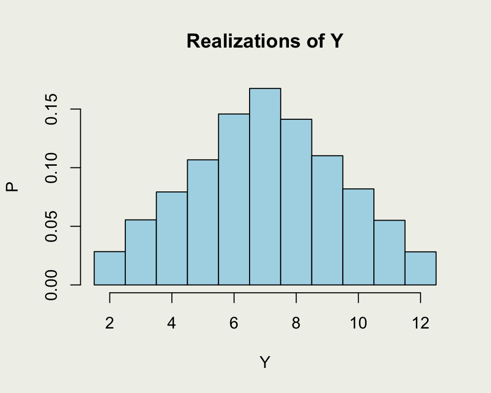
This is a more direct demonstration of random draws from a distribution of \(Y = X_1 + X_2\)
Bivariate Case
- Marginalization
\[ f_Y(y) = \int_{-\infty}^\infty f_{X,Y}(x, y) \, \mathrm{d}x. \]
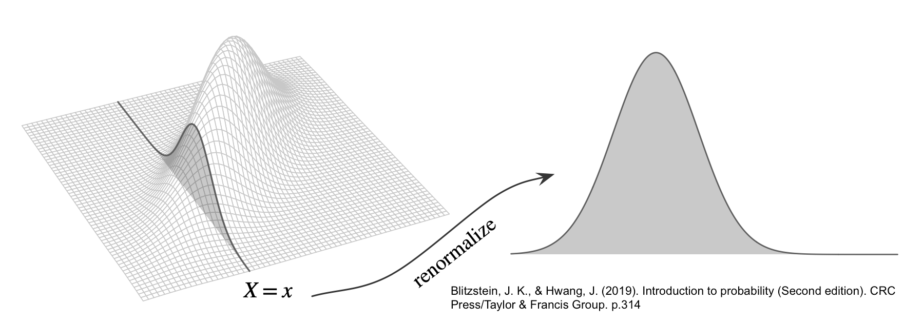
- Conditional CDF
\[ F_{Y \mid X}(y \mid x) = \P(Y \leq y \mid X = x) \]
- Conditional PDF: a function of \(y\) for fixed \(x\) \[ f_{Y|X}(y \mid x) = \frac{f_{X,Y}(x, y)}{f_X(x)} \]
Joint, Marginal, and Conditional
- What is \(\P(G = m \mid S = y)\), probability of being
male given survival? - To compute that, we only consider the column
where Survival = Yes - \(\P(G = m \mid S = y) = \frac{\P(G = m \, \cap \, S = y)}{\P(S = y)} = \frac{0.167}{0.323} \\ \approx 0.52\)
- You want \(\P(S = y \mid G = m)\), comparing it to \(\\ \qquad \ \ \ \ \ \ \P(S = y \mid G = f)\)
- \(\P(S = y \mid G = m) = \frac{\P(G = m \, \cap \, S = y)}{\P(G = m)} = \frac{0.167}{0.787} \\ \approx 0.21\)
- \(\P(S = y \mid G = f) = \frac{\P(G = f \, \cap \, S = y)}{\P(G = f)} = \frac{0.156}{0.213} \\ \approx 0.73\)
- How would you compute \(\P(S = n \mid G = m)\)?
- \(\P(S = n \mid G = m) = 1 - \P(S = y \mid G = m)\)
| Sex | No | Yes | Total |
|---|---|---|---|
| Male | 0.620 | 0.167 | 0.787 |
| Female | 0.057 | 0.156 | 0.213 |
| Total | 0.677 | 0.323 | 1.000 |
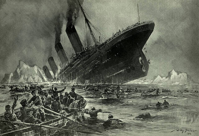 “Untergang der Titanic”, as conceived by Willy Stöwer, 1912
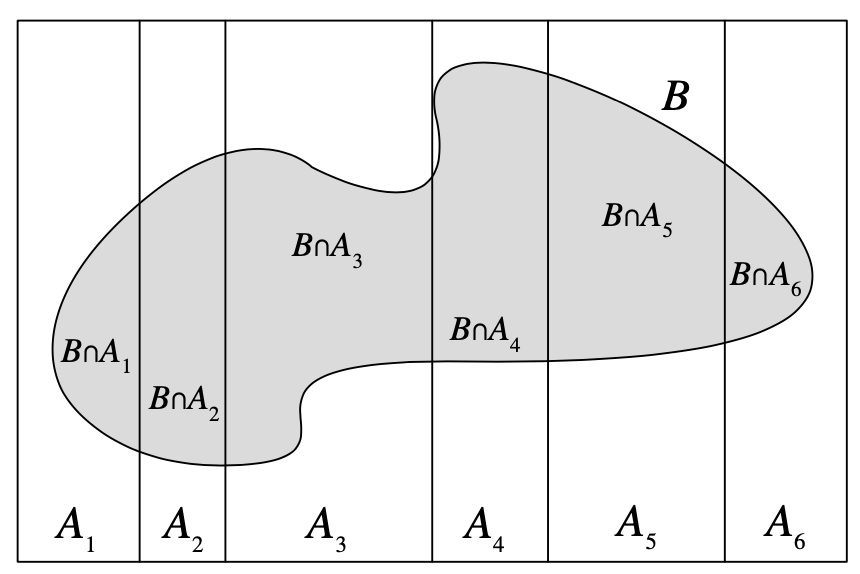
Law of Total Probability (LOTP)
Let \(A\) be a partition of \(\Omega\), so that each \(A_i\) is disjoint, \(\P(A_i >0)\), and \(\cup A_i = \Omega\). \[ \P(B) = \sum_{i=1}^{n} \P(B \cap A_i) = \sum_{i=1}^{n} \P(B \mid A_i) \P(A_i) \]
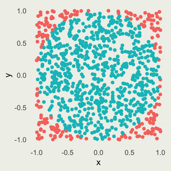
Estimating \(\pi\) by Simulation
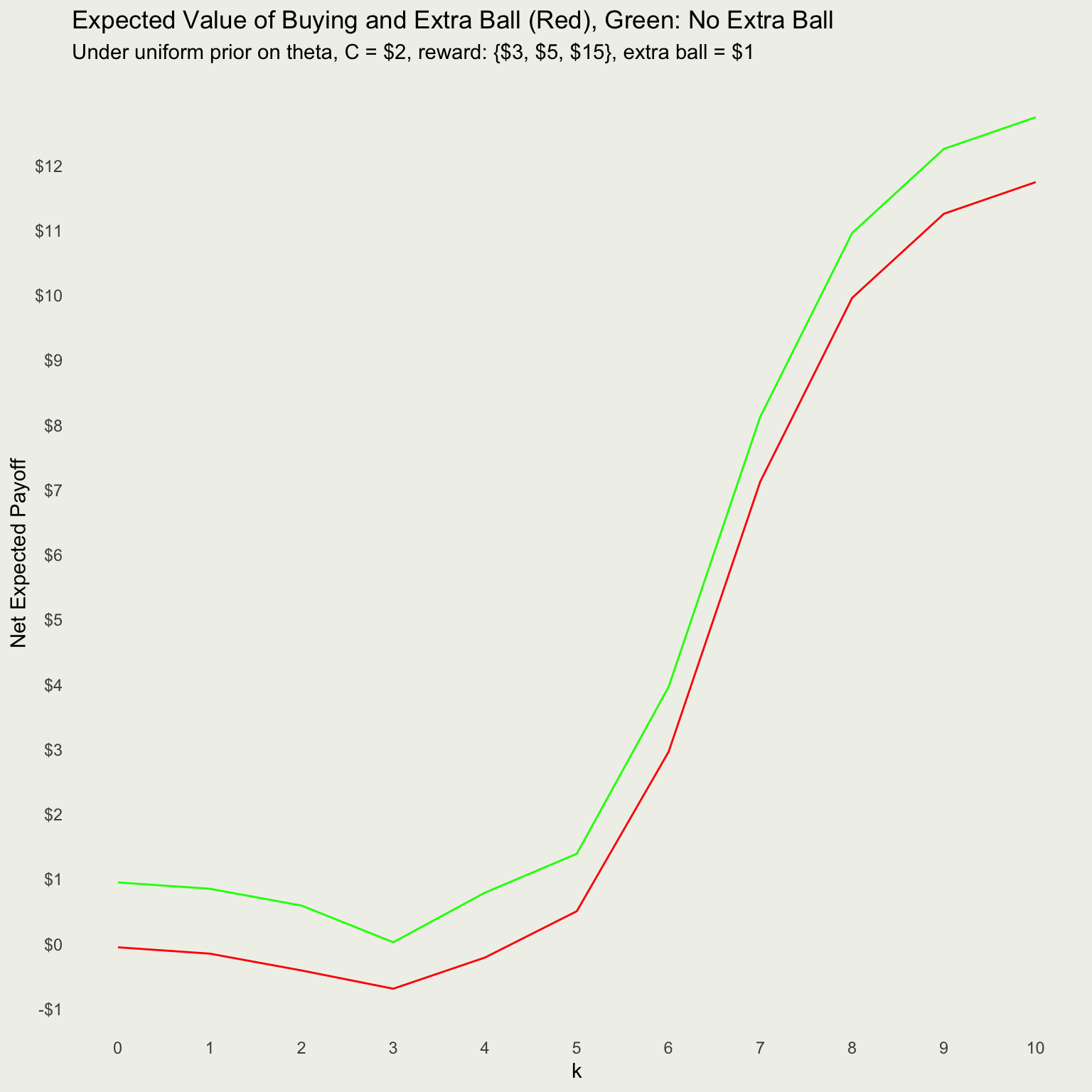
Mystery Box Game Analysis
- Game Setup:
- You are offered to bet on the proportion of red balls in a box
- True proportions: \(\theta \in \{0.25,\, 0.50,\, 0.75\}\)
- You are allowed to draw 10 balls from the box with replacement
- Payoffs if your chosen \(\theta\) is correct:
- For \(\theta=0.25\): $3
- For \(\theta=0.50\): $5
- For \(\theta=0.75\): $15

- Your options are: A) Don’t play; B) Draw 10 balls, and pay $2 to play; C) Pay $1 to buy an extra ball (11th), then pay $2 to play
- Warmup: Before drawing 10 balls what is the expected value of each bet? Which one should we choose? (still have to pay $2 to play)
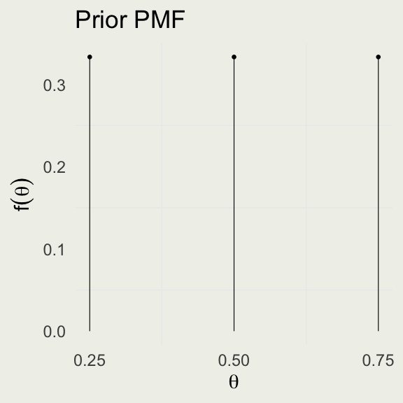
Example Prior Model
- What does it mean to put a uniform prior on \(\theta\)?
- What are we assuming about the game design under this prior?
- Is that a reasonable assumption, given the payoffs?
- We take one ball from the box; what is \(\P(y = \text{red})\)?
- Law of Total Probability (LOTP):
\[ \begin{eqnarray*} \P(y = \text{red}) &=& \sum_{i=1}^{3} f(y = \text{red}, \theta_i) = \sum_{i=1}^{3} f(y = \text{red} \mid \theta_i) f(\theta_i) \\ &=& (0.25) \cdot \left(\frac{1}{3}\right) + (0.50) \cdot \left(\frac{1}{3}\right) + (0.75) \cdot \left(\frac{1}{3}\right) \end{eqnarray*} \]
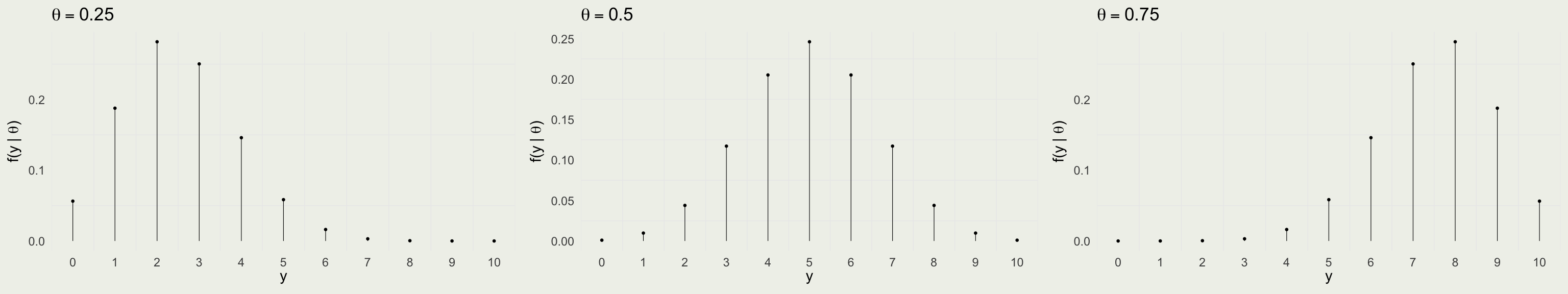
Data Model: Before Drawing 10 Balls
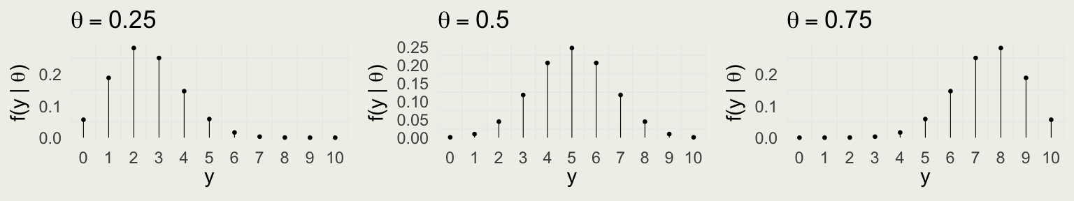
Take red ball as success, so \(y\) successes out of \(N = 10\) trials \[ y | \theta \sim \text{Bin}(N,\theta) = \text{Bin}(10,\theta) \]
\(f(y \mid \theta) = \text{Bin} (y \mid 10,\theta) = \binom{10}{y} \theta^y (1 - \theta)^{10 - y}\) for \(y \in \{0,1,\ldots,10\}\)
Is this a valid probability distribution as a function of \(y\)?
Visualizing the Likelihood Function
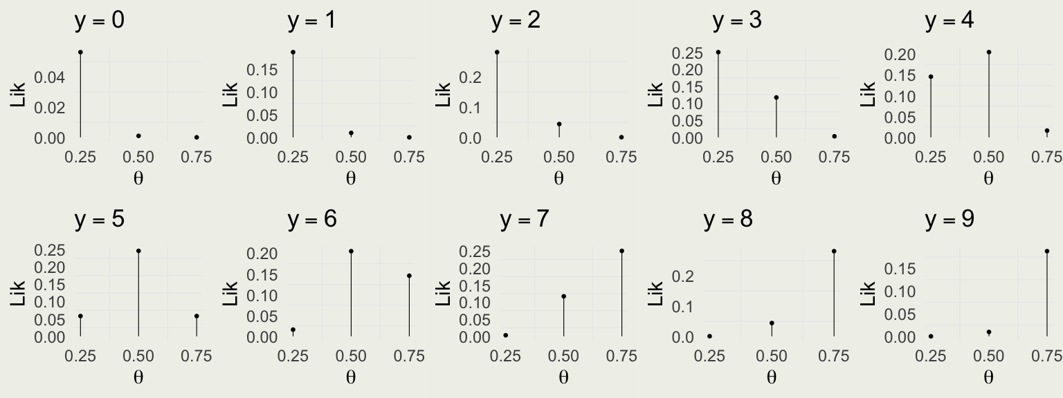
Compare with the data model:
What About For All Possible Outcomes?
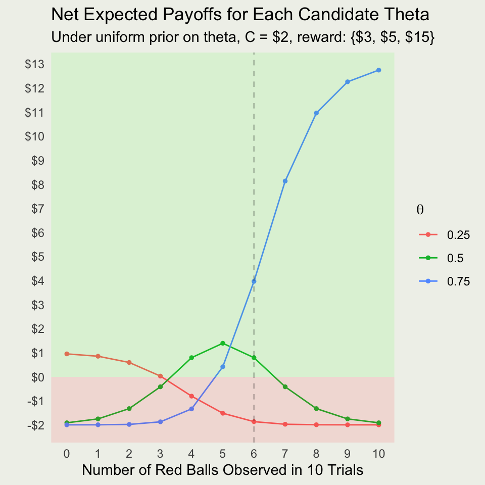
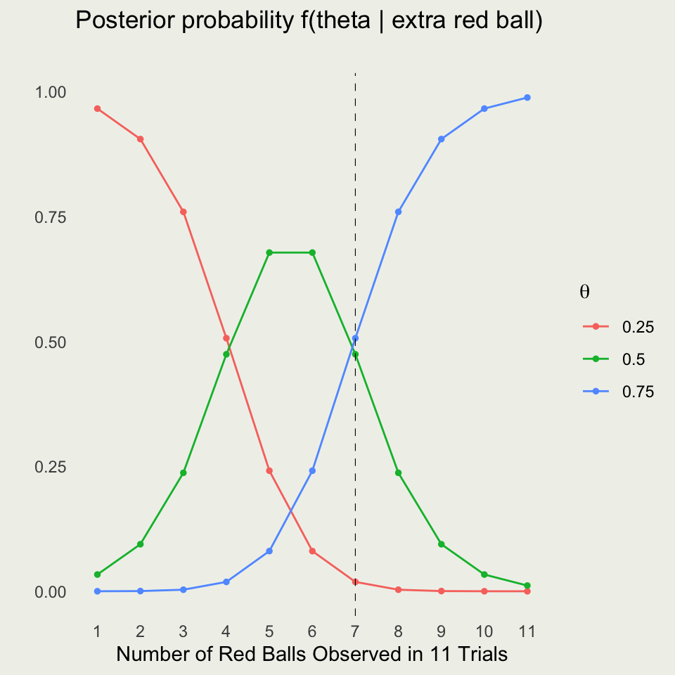
Net Payoffs With and Without Extra Ball?