Bayesian Inference

NYU Applied Statistics for Social Science Research

Eric Novik | Spring 2024 | Lecture 2

Conjugate models and Beta-Binomial

Bayesian workflow
Beta distribution
Great expectations
Tuning the prior model for the clinical trial analysis
Binomial likelihood with continuous \(\theta\)
Deriving the conjugate posterior
Analysis of the sex ratio
Compromise between priors and data model
Coherence of Bayesian inference

\[ \DeclareMathOperator{\E}{\mathbb{E}} \DeclareMathOperator{\P}{\mathbb{P}} \DeclareMathOperator{\V}{\mathbb{V}} \DeclareMathOperator{\L}{\mathcal{L}} \DeclareMathOperator{\I}{\text{I}} \DeclareMathOperator*{\argmax}{arg\,max} \DeclareMathOperator*{\argmin}{arg\,min} \]

Homework

How did you find the homework?
Homework review

Bayesian Workflow

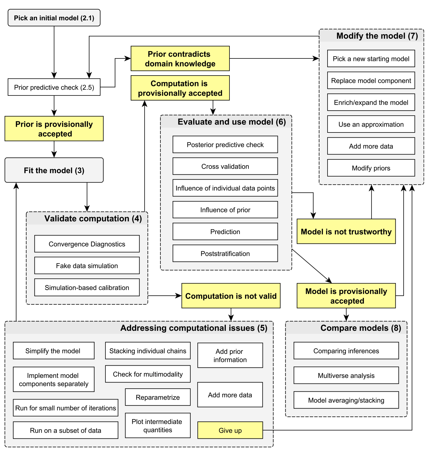
Statistics is like building a bridge — we first simulate the conditions under which our bridge should withstand various forces, then we build a bridge, and once built, we test it before letting people drive on it.
Prior knowledge (not just prior distributions) here would be strength properties of concrete, optimal shape for the length, expected wind conditions, expected load of traffic, and maybe even expected momentum (mass * velocity) of an out-of-control tanker ramming into one of the supporting columns. The more important our “bridge,” the more testing we do.

Bayesian Inference vs Bayesian Workflow¹

Bayesian inference is concerned with computing \(f(\theta \mid y) \propto f(\theta) f(y \mid \theta)\)
Bayesian workflow covers all aspects of data analysis:
- Gather prior information
- Build the initial model
- Run an inference algorithm (Bayesian inference)
- Add model complexity, try a different model, perform model selection
- Make a decision

Why do we need workflow

Following the principle of engineering, we start with a simple model
It will likely fit the data (no guarantees) and will not take too long to run
The simple model will likely not be very good, but now we:
- Have a straw man against which better models can be evaluated
- Can code the full cycle of data selection, model build, model test, and model diagnostics
We gradually add components and rerun the tests
If data are large, we can subsample the data to test our model

We want to compare models as we add features
We calibrate this workflow, including a selection of the inference algorithm based on cost of being wrong

On with the show…

Last time, we presented the discretized version of the prior
In practice, we are typically working in continuous space
In general, the prior model can be arbitrarily complex
There is a family of distributions called the exponential family, for which the prior has the same kernel as the posterior
This is called conjugacy
In practice, we seldom rely on conjugate relationships
Beta distribution is conjugate to Binomial

Continous Probability Distributions

Recall that for the continuous RVs we have, the CDF is defined as \[ \begin{eqnarray} F(x) & = & \int_{-\infty}^{x} f(t) \, \text{d}t, \, \text{and} \\ f(x) & = & \frac{\text{d}}{\text{d}x}F(x), \, \text{where } F \text{ is differentiable} \end{eqnarray} \]
To compute event probabilities: \[ \begin{eqnarray} \P(a \le X \leq b) & = & F(b) − F(a) = \int_{a}^{b} f(x) \, \text{d}x \\ \P(X \in A) & = & \int_{A} f(x) \, \text{d}x \end{eqnarray} \]
As in the case of PMFs: \[ \begin{eqnarray} f(x) \geq 0 \\ \int_{-\infty}^{\infty} f(x) \, \text{d}x = 1 \end{eqnarray} \]

Introducing Beta

Beta distribution has the following functional form for \(\alpha > 0, \, \beta > 0, \, \theta \in (0, 1)\) \[ \begin{eqnarray} \text{Beta}(\theta \mid \alpha,\beta) & = & \frac{1}{\mathrm{B}(\alpha,\beta)} \, \theta^{\alpha - 1} \, (1 - \theta)^{\beta - 1} \\ \text{B}(a,b) \ & = & \ \int_0^1 u^{a - 1} (1 - u)^{b - 1} \, \text{d}u \ \\ & = & \ \frac{\Gamma(a) \, \Gamma(b)}{\Gamma(a+b)} \\ \Gamma(x) & = & \int_0^{\infty} u^{x - 1} \exp(-u) \, \text{d}u \end{eqnarray} \]

factorial(0:9)

 [1]      1      1      2      6     24    120    720   5040  40320 362880

gamma(1:10)

 [1]      1      1      2      6     24    120    720   5040  40320 362880

For positive integrers \(n\): \(\, \Gamma(n+1) = n!\) and in general \(\Gamma(z + 1) = z \Gamma(z)\)
\(\text{Beta}(1, 1)\) is equivalent to \(\text{Unif(0, 1)}\). Why? (work it out)

Visualizing Beta

The mode of Beta, \(\text{Mode}(\theta) = \argmax_\theta \text{Beta}(\theta \mid \alpha, \beta)\) is shown in red and the function maximum in blue

Expectations

Recall the definition of expectations for continuous random variables
We often write \(\mu\) or \(\mu_X\) for expected value of \(X\) \[ \mu_X = \E(X) = \int x \cdot f(x) \, \text{d}x \]
Variance is a type of expectation, which we often denote by \(\sigma^2\) \[ \sigma_X = \V(X) = \E(X - \mu)^2 = \int (X - \mu)^2 f(x) \, \text{d}x \]
It is often more convenient to write the variance as \[ \V(X) = \E(X^2) - \mu^2 \]

What to expect from Beta

Keeping in mind that a Gamma function is a continuous analog of the factorial:

\[ \begin{eqnarray} \E(\theta) &=& \int_{0}^{1} \frac{1}{\mathrm{B}(\alpha,\beta)} \, \theta \cdot \theta^{\alpha - 1} \, (1 - \theta)^{\beta - 1} \, \text{d}\theta \\ &=& \frac{1}{\mathrm{B}(\alpha,\beta)}\int_{0}^{1} \color{red}{\theta^\alpha \, (1 - \theta)^{\beta - 1}} \, \text{d}\theta \\ \end{eqnarray} \]

\[ \begin{eqnarray} &=& \frac{\Gamma(\alpha + \beta)}{\Gamma(\alpha) \, \Gamma(\beta)} \cdot \color{red}{\frac{\Gamma(1 + \alpha) \Gamma(\beta)}{\Gamma(1 + a + b)}} \\ &=& \frac{\Gamma(\alpha + \beta)}{\Gamma(\alpha)} \cdot \frac{\Gamma(1 + \alpha)}{\Gamma(1 + \alpha + \beta)} \\ &=& \frac{\Gamma(\alpha + \beta)}{\Gamma(\alpha)} \cdot \frac{a \Gamma(\alpha)}{(\alpha + \beta) \Gamma(\alpha + \beta)} \\ &=& \frac{\alpha}{\alpha + \beta} \end{eqnarray} \]

What is the value of \(\int_{0}^{1} \, \theta^\alpha \, (1 - \theta)^{\beta} \, d\theta\)

What to expect from Beta

We can find the mode of this distribution by taking the log, differentiating with respect to \(\theta\), and setting the derivative function to zero \[ \begin{eqnarray} \E(\theta) & = & \frac{\alpha}{\alpha + \beta} \\ \text{Mode}(\theta) & = & \frac{\alpha - 1}{\alpha + \beta - 2} \;\; \text{ when } \; \alpha, \beta > 1. \\ \end{eqnarray} \]
The variance of \(\theta\) can be derived using the definition of the variance operator \[ \begin{eqnarray} \V(\theta) & = & \frac{\alpha \beta}{(\alpha + \beta)^2(\alpha + \beta + 1)} \end{eqnarray} \]
Notice when \(\alpha = \beta\), \(\E(\theta) = \text{Mode}(\theta)\)

Example: Placenta Previa

We borrow an example from BDA3: the probability of girl birth given placenta previa (PP)
Placenta previa is a condition when the placenta completely or partially covers the opening of the uterus
A PP study in Germany found that out of 980 births, 437 or \(\approx 45\%\) were female
Sex ratio in the population has been stable over space and time at 48.5% females with deviations within no more than 1%¹
Our task is to assess the evidence for \(\P(\text{ratio} < .485 \mid \text{PP})\)

Biomomial Likelihood

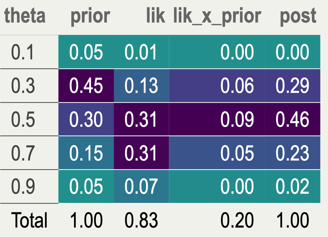
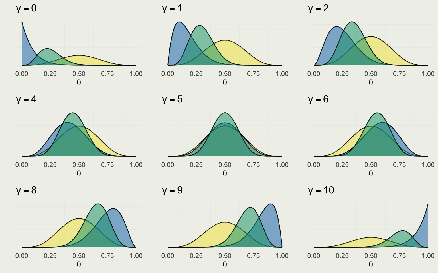
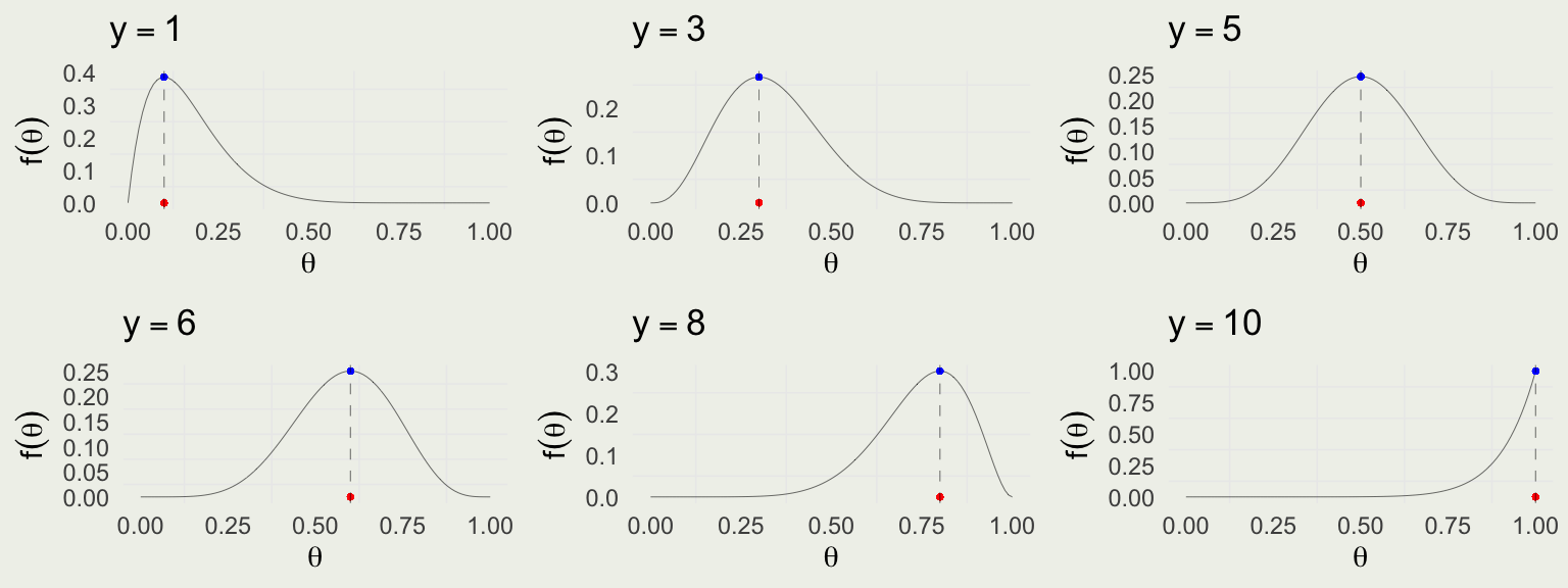
Recall that Likelihood is the function of the parameter \(\theta\), assuming \(\theta \in [0,1]\) \[ \text{Bin}(y \mid \theta) = \binom{N}{y} \theta^y (1 - \theta)^{N - y} \propto \theta^y (1 - \theta)^{N - y} \]
Assuming \(N = 10\), the likelihood for \(\theta\), given a few possible values of \(y\) successes

Deriving the Posterior Distribution

The denominator is constant in \(\theta\); we will derive the posterior up to a proportion \[ \begin{eqnarray} f(y \mid \theta) & \propto & \theta^y (1 - \theta)^{N - y} \\ f(\theta) & \propto & \theta^{\alpha - 1} \, (1 - \theta)^{\beta - 1} \\ f(\theta \mid y) & \propto & f(y \mid \theta) f(\theta) \\ & = & \theta^y (1 - \theta)^{N - y} \cdot \theta^{\alpha - 1} \, (1 - \theta)^{\beta - 1} \\ & = & \theta^{y + \alpha - 1} (1 - \theta)^{N - y + \beta - 1} \\ f(\theta \mid y) & = & \text{Beta}(\alpha + y, \,\beta + N - y) \end{eqnarray} \]
\(f(\theta)\): \(\alpha - 1\) prior successes and \(\beta - 1\) prior failures
The last equality comes from matching the kernel \(\theta^{y + \alpha - 1} (1 - \theta)^{N - y + \beta - 1}\) to the normalized Beta PDF which has a normalizing constant \(\frac{\Gamma (\alpha +\beta + N)}{\Gamma (\alpha + y) \Gamma (\beta + N - y)}\)
Since the posterior is in the same family as the prior, we say that Beta is conjugate to Binomial

Posterior Expectations

\[ \begin{eqnarray} \E(\theta \mid y) & = & \frac{\alpha + y}{\alpha + \beta + n} = \frac{\alpha + \beta}{\alpha + \beta + n}\cdot \E(\theta) + \frac{n}{\alpha + \beta + n}\cdot\frac{y}{n} \\ \V(\theta \mid y) & = & \frac{(\alpha + y)(\beta + n - y)}{(\alpha + \beta + n)^2(\alpha + \beta + n + 1)} \\ \text{Mode}(\theta \mid y) & = & \frac{\alpha + y - 1}{\alpha + \beta + n - 2} = \frac{\alpha + \beta - 2}{\alpha + \beta + n - 2} \cdot\text{Mode}(\theta) + \frac{n}{\alpha + \beta + n - 2} \cdot\frac{y}{n} \end{eqnarray} \]

Note that the posterior expectation is between \(y/n\) and \(\frac{\alpha}{\alpha + \beta}\)
Also note that as sample becomes very large \(\E(\theta \mid y) \rightarrow \frac{y}{n}\) and \(\V(\theta \mid y) \rightarrow 0\)
As before, \(\text{Mode}(\theta \mid y) = \E(\theta \mid y)\), when \(\alpha = \beta\)

Variance Reduction Rate

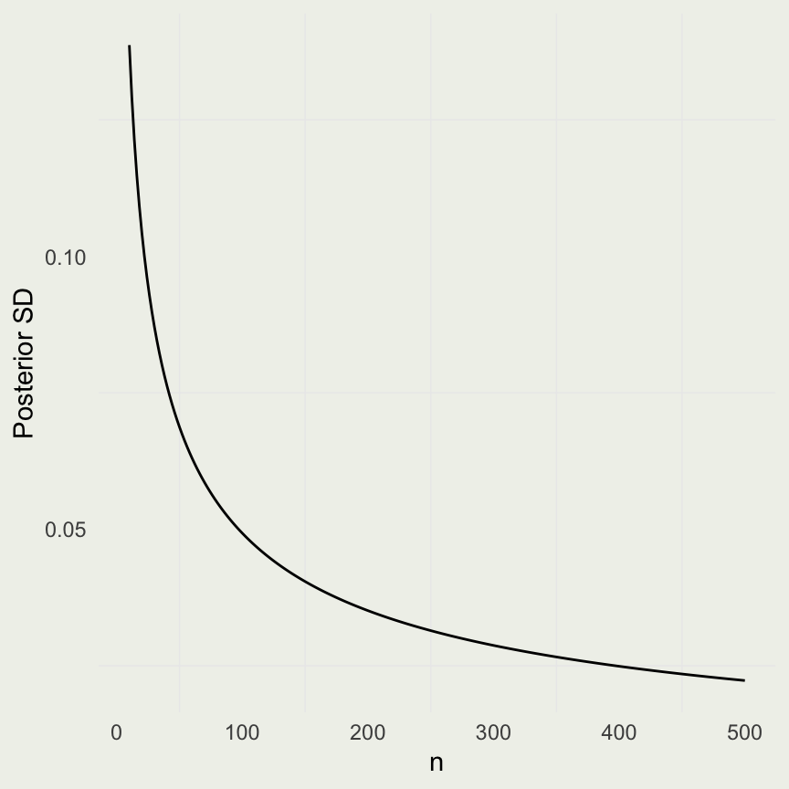
post_v <- function(a, b, y, n) {
  ((a + y) * (b + n - y)) / ((a + b + n)^2 * (a + b + n + 1))
}
n <- seq(10, 500, by = 2)
y <- 1:246
v <- post_v(1, 1, y = y, n = n)
ggplot(aes(n, v), data = data.frame(n, v)) +
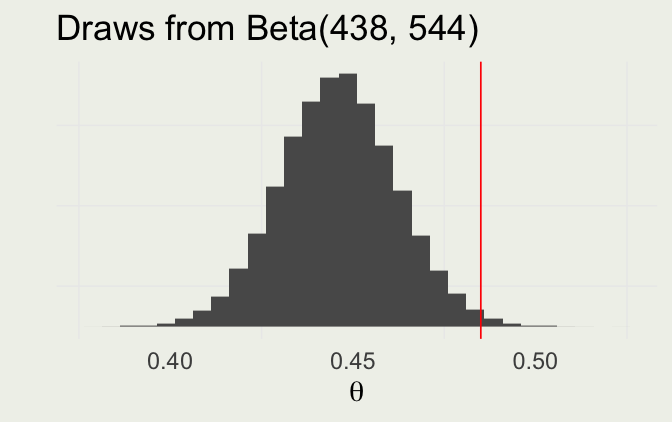
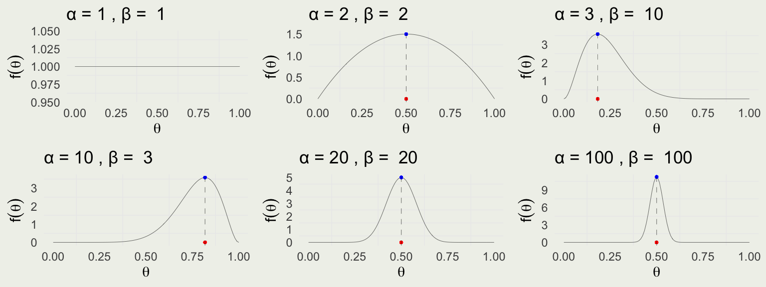
  geom_line() + ylab("Var")

Example: Placenta Previa

Let’s derive the analytical posterior and compare it with the samples from the posterior distribution
First, we will consider the uniform \(\text{Beta}(1, 1)\) prior
We are told that data are \(N = 980\) and \(y = 437\) female births
The posterior is \(\text{Beta}(1 + 437, 1 + 980 - 437) = \text{Beta}(438, 544)\)
\(\E(\theta \mid Y=437) = \frac{\alpha + 437}{\alpha + \beta + 980} = \frac{438}{982} \approx 0.446\)
\(\sqrt{\V(\theta \mid Y=y)} \approx\) 0.016

int <- 0.95; l <- (1 - int)/2; u <- 1 - l
upper <- qbeta(u, 438, 544) |> round(3)
lower <- qbeta(l, 438, 544) |> round(3)
cat("95% posterior interval is [", lower, ", ", upper, "]", sep = "")

95% posterior interval is [0.415, 0.477]

event_prob <- integrate(dbeta, lower = 0, upper = 0.485, shape1 = 438, shape2 = 544)[[1]]
cat("Probability that the ratio < 0.485 under uniform prior =", round(event_prob, 3))

Probability that the ratio < 0.485 under uniform prior = 0.993

pbeta(0.485, shape1 = 438, shape2 = 544) |> round(3)

[1] 0.993

Obtaining Quantiles by Sampling

We can use R’s rbeta() RNG to generate draws from the posterior

draws <- rbeta(n = 1e5, 438, 544)
p <- ggplot(aes(draws), data = data.frame(draws))
p + geom_histogram(bins = 30) + ylab("") +
  geom_vline(xintercept = 0.485, 
             colour = "red", size = 0.3) +
  ggtitle("Draws from Beta(438, 544)") + 
  theme(axis.text.y = element_blank()) + 
  xlab(expression(theta))

We can use the quantile() function to get the posterior interval and compute the event probability by evaluating the expectation of the indicator function as before

quantile(draws, probs = c(0.025, 0.5, 0.975)) |> round(3)

 2.5%   50% 97.5% 
0.415 0.446 0.477

cat("Probability that the ratio < 0.485 under uniform prior =", mean(draws < 0.485) |> round(3))

Probability that the ratio < 0.485 under uniform prior = 0.993

Population Priors

What priors should we use if we think the sample is drawn from the sex ratio “hyper-population”?
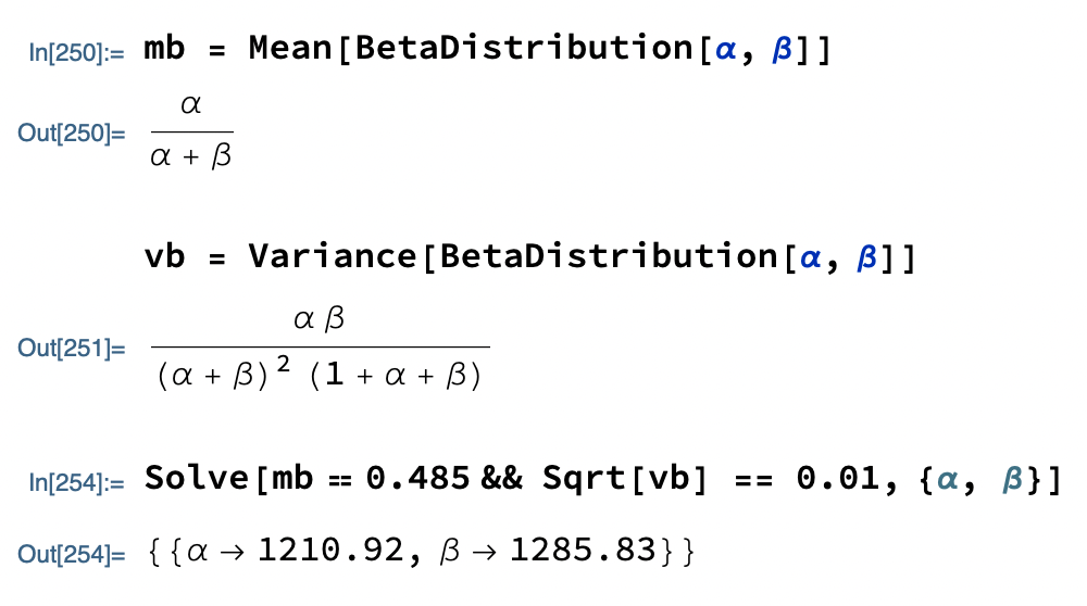
We know that the population mean is 0.485 and the standard deviation is about 0.01
Back out the parameters of the population Beta distribution

\[ \begin{eqnarray} \begin{cases} \frac{\alpha}{\alpha + \beta} & = & 0.485 \\ \sqrt{\frac{\alpha \beta}{(\alpha + \beta)^2(\alpha + \beta + 1)}} & = & 0.01 \end{cases} \end{eqnarray} \]

\(\alpha \approx 1211\) and \(\beta \approx 1286\)

Check the result with the simulation

x <- rbeta(1e4, 1211, 1286)
mean(x) |> round(3)

[1] 0.485

sd(x) |> round(3)

[1] 0.01

We can let Mathematica do the algebra

Posterior with Population Priors

\(f(\theta | y) = \text{Beta}(1211 + 437, 1286 + 543) = \text{Beta}(1648,1829)\)
We can compare the prior and posterior using summarize_beta_binomial() in the bayesrules package

library(bayesrules)
summarize_beta_binomial(alpha = 1211, beta = 1286, y = 437, n = 980)

      model alpha beta      mean      mode          var          sd
1     prior  1211 1286 0.4849820 0.4849699 9.998978e-05 0.009999489
2 posterior  1648 1829 0.4739718 0.4739568 7.168560e-05 0.008466735

int <- 0.95; l <- (1 - int)/2; u <- 1 - l
upper <- qbeta(u, 1648, 1829) |> round(3)
lower <- qbeta(l, 1648, 1829) |> round(3)
cat("95% posterior interval is [", lower, ", ", upper, "]", sep = "")

95% posterior interval is [0.457, 0.491]

event_prob <- pbeta(0.485, shape1 = 1648, shape2 = 1829)
cat("Probability that the ratio < 0.485 under population prior =", round(event_prob, 3))

Probability that the ratio < 0.485 under population prior = 0.904

Under uniform prior 95% posterior interval was [0.415, 0.477]
And probability that the ratio < 0.485 under uniform prior = 0.993

Visualizing Bayesian Rebalancing

The following uses \(\text{Beta}(5, 5)\) prior and N = 10. Guess what color is likelihood, prior, and posterior.

Data Order and Batch Invariance

In Bayesian analysis, we can update all at once or one datum at a time and everything in between and in any order (assuming exchangeable observations)
This is a general result, not just for Beta Binomial (see Section 4.5)
In practice, when we don’t have analytic posteriors, this is not so easy to do
Suppose we observe \(y = y_1 + y_2\) and \(N = N_1 + N_2\) trials all at once
For all at once case, the posterior is in \(f(\theta \mid y) = \text{Beta}(\alpha + y, \,\beta + N - y)\) as before
Now, suppose we observe \(y_1\) successes in \(n_1\) trials first
The posterior is \(f(\theta \mid y_1) = \text{Beta}(\alpha + y_1, \,\beta + N_1 - y_1)\)
We now observe, \(y_2\) successes in \(n_2\) trials. The posterior is \(f(\theta \mid y= y_1 + y_2) = \text{Beta}(\alpha + y_1 + y_2, \,\beta + N_1 - y_1 + N_2 - y_2)\\ = \text{Beta}(\alpha + y, \,\beta + N - y)\)

General Case

Suppose we observe data point \(y_1\), and then data point \(y_2\)¹

\[ \begin{eqnarray} f(\theta \mid y_1) &=& \frac{f(\theta)f(y_1 \mid \theta)}{f(y_1)} \\ f(\theta \mid y_2) &=& \frac{\frac{f(\theta)f(y_1 \mid \theta)}{f(y_1)} f(y_2 \mid \theta)}{f(y_2)} \\ &=& \frac{f(\theta)f(y_1 \mid \theta) f(y_2 \mid \theta)}{f(y_1)f(y_2)} \end{eqnarray} \]

Observing data point \(y_2\), and then data point \(y_1\), will results in the same distribution
What if we observed both points at once?

\[ \begin{split} f(\theta \mid y_1,y_2) & = \frac{f(\theta)f(y_1,y_2 \mid \theta)}{f(y_1)f(y_2)} \\ & = \frac{f(\theta)f(y_1 \mid \theta)f(y_2 \mid \theta)}{f(y_1)f(y_2)} \end{split} \]

The myth of objectivity in science

All of science requires choices, and those choices are, by definition, subjective
Neither Frequentist nor Bayesian inference imbues objectivity into your analysis
All priors are subjective, including no priors, which don’t exist (uniform prior on the real line is not “no prior”)
Remember that important scientific discoveries were made before Statistics became a thing
A better alternative to objective vs subjective debate:

…objectivity replaced by transparency, consensus, impartiality, and correspondence to observable reality, and subjectivity replaced by awareness of multiple perspectives and context dependence¹

Bayesian Inference

Conjugate models and Beta-Binomial

Homework

Bayesian Workflow

Bayesian Inference vs Bayesian Workflow1

Why do we need workflow

On with the show…

Continous Probability Distributions

Introducing Beta

Visualizing Beta

Expectations

What to expect from Beta

What to expect from Beta

Example: Placenta Previa

Biomomial Likelihood

Deriving the Posterior Distribution

Posterior Expectations

Variance Reduction Rate

Example: Placenta Previa

Obtaining Quantiles by Sampling

Population Priors

Posterior with Population Priors

Visualizing Bayesian Rebalancing

Data Order and Batch Invariance

General Case

The myth of objectivity in science

Bayesian Inference vs Bayesian Workflow¹