metropolis_iteration_1 <- function(y, current_mean, proposal_scale,
sd, prior_mean, prior_sd) {
# assume prior ~ N(prior_mean, prior_sd) and sd is known
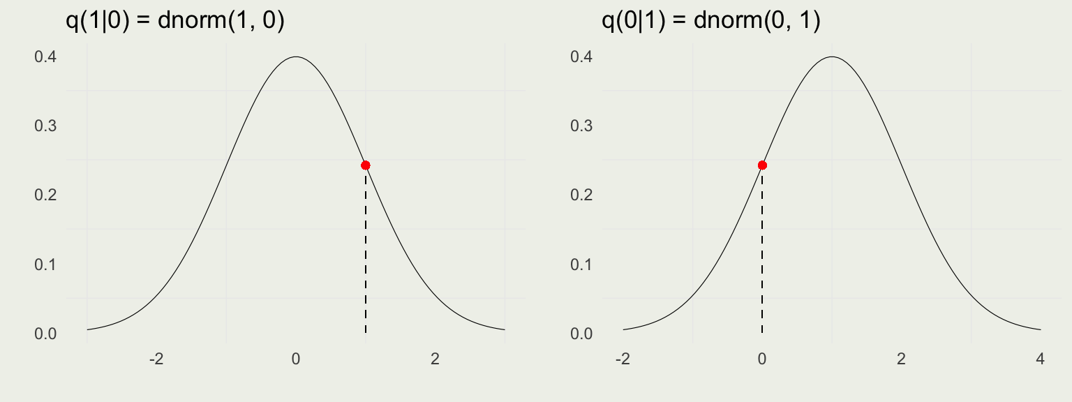
# proposal sampling distribution q = N(current_mean, proposal_scale)
proposal_mean <- rnorm(n = 1, mean = current_mean, sd = proposal_scale) # q(mu' | mu)
f_proposal <- dnorm(proposal_mean, mean = prior_mean, # proposal prior, f(theta')
sd = prior_sd) *
dnorm(y, mean = proposal_mean, sd = sd) # proposal lik, f(y | theta')
f_current <- dnorm(current_mean, mean = prior_mean, # current prior, f(theta)
sd = prior_sd) *
dnorm(y, mean = current_mean, sd = sd) # current lik, f(y | theta)
ratio <- f_proposal / f_current # [f(theta') * f(y | theta')] / [f(theta) * f(y | theta)]
alpha <- min(ratio, 1)
if (alpha > runif(1)) { # this is just another way of flipping a coin
next_value <- proposal_mean
} else {
next_value <- current_mean
}
return(next_value)
}

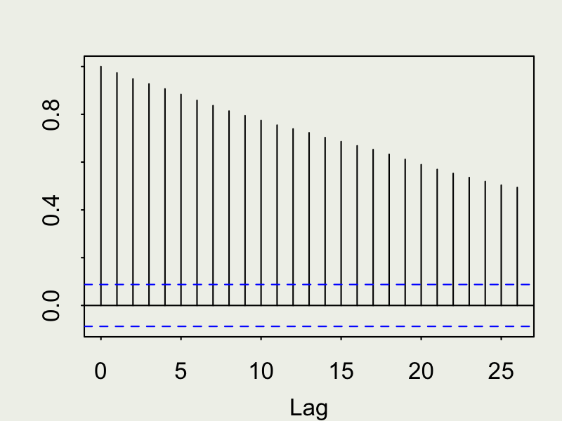
 Autocorrelation function (ACF)
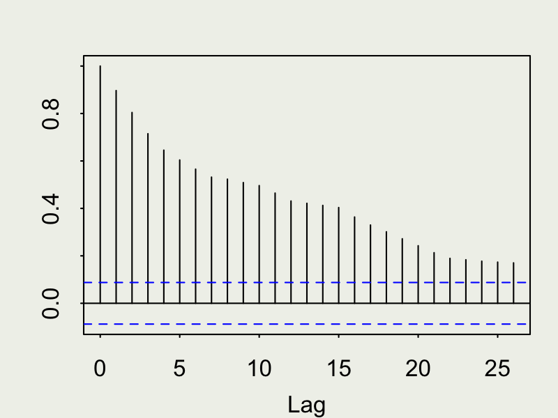