From Entropy to Model Evaluation and LOO-CV

This case study is based on Practical Bayesian model evaluation using leave-one-out cross-validation and WAIC (Vehtari, Gelman, and Gabry 2017) and Information Theory, Inference and Learning Algorithms (MacKay 2003).

\[ \DeclareMathOperator{\E}{\mathbb{E}} \DeclareMathOperator{\d}{text{d}} \DeclareMathOperator{\P}{\mathbb{P}} \DeclareMathOperator{\V}{\mathbb{V}} \DeclareMathOperator{\L}{\mathcal{L}} \DeclareMathOperator{\I}{\text{I}} \DeclareMathOperator*{\argmax}{arg\,max} \DeclareMathOperator*{\argmin}{arg\,min} \]

Before discussing LOO-CV, it is helpful to to review the its information-theoretic justification for model selection. We will start with the concept of information entropy and cross-entropy that will lead is to relative enrtopy, which also goes by the name of KL divergence (KLD) and finally to how minimizing KLD naturally leads to LOO-CV.

Entropy

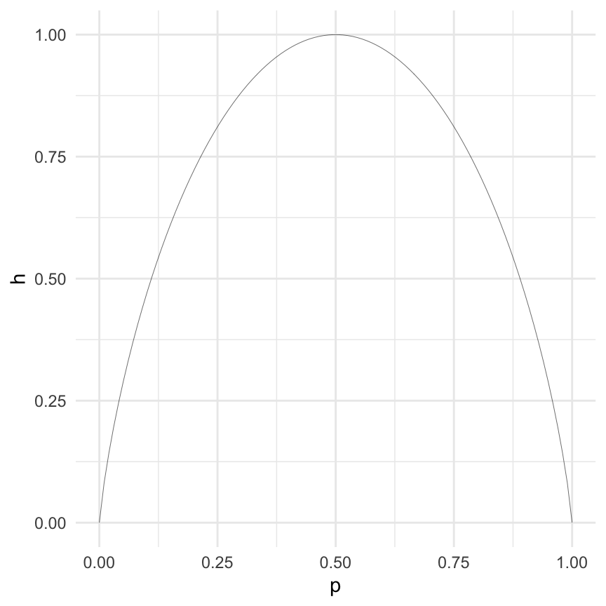
Entropy is sometimes decribed as a measure of disorder in a system, but this is not a very helpful description. One way to think of information entropy is a measure of surprise. Let’s take a simple system that can either be in state 0 or state 1. If every time we observe the system it is either state 1 or 0 and never changes, we can’t be surp rised by what we see, or another way of saying that is that this system can only be arranged in one way, so our surprise or entropy is 0 in either case. Suppose that the system can be state 1 (or 0) with probability of \(p = 1/2\). In this case, my surprise should be at its maximum, compared with any other value of \(p\).

Let’s take a particular PMF for this Bernoulli with \(p(X = 1) = 0.9\) and \(p(X = 2) = 0.1\). Shannon called the information content of X = 1 of this system:

\[ h(x) = \log_2 \frac{1}{p(x)} = -\log_2(p(x)) \] \(h(1) \approx 0.15 \text{ and } h(0) \approx 3.32\)

This function has a property that the higher the probability (of seeing 1), the lower is the surprise that you see it.

library(purrr)
library(dplyr)
library(ggplot2)

H <- function(p) {
# p is a PMF expressed as a row vector
# compute H(x) = sum(p(x) * log2(1 / p(x)))
  N <- length(p)
  H <- numeric(N)
  for (n in 1:N) {
    if (p[n] == 0) {
      H[n] <- 0
    } else {
      H[n] <- -p[n] * log2(p[n]) 
    }
  }
  return(sum(H))
}
p <- seq(0, 1, len = 100)
p <- data.frame(p = p, q = 1 - p)
p <- p |>
  rowwise() |>
  mutate(h = H(c_across(everything()))) |>
  ungroup()

ggplot(aes(x = p, y = h), data = p) +
  geom_line(linewidth = 0.1) + theme_minimal()

KL Divergence

The theoretical justification of the methods described in this case study has it’s underpinnnings in information theory measuring distance between distribution called Kullback–Leibler divergence that is sometimes called relative entropy. Suppose \(P\) is the true distribution with PDF \(p(y)\). We want to know how close in KL sense \(Q\) with PDF \(q(y)\) is to \(P\). KL is not a metric since \(D_{\mathrm{KL}}(P \,\|\, Q) \ne D_{\mathrm{KL}}(Q \,\|\, P)\).

\[ \begin{eqnarray} D_{\mathrm{KL}}(P\|Q) &=& \mathbb{E}_{Y\sim P}\!\biggl[\log \!\biggl( \frac{p(Y)}{q(Y)} \biggr) \biggr] \\ &=& \int p(y)\,\log\!\biggl(\frac{p(y)}{q(y)}\biggr)\,\text{d}y \end{eqnarray} \]

As an exmaple suppose \(P\) is \(\text{Normal}(0, 1)\) and Q is \(\text{Normal}(\mu, 1)\). We will compute the expectation using SymPy.

import sympy as sp

y, μ = sp.symbols('x μ', real=True)

p = 1/sp.sqrt(2*sp.pi) * sp.exp(-y**2/2)
q = 1/sp.sqrt(2*sp.pi) * sp.exp(-(y - μ)**2/2)

integrand = p * sp.log(p/q)
kl = sp.integrate(integrand, (y, -sp.oo, sp.oo))
kl = sp.simplify(kl)

latex_expr = "$$" + "D_{\\text{KL}}(\\text{Normal}(0, 1) \| \\text{Normal}(\mu, 1)) = " + sp.latex(kl) + "$$"
print(latex_expr)

\[D_{\text{KL}}(\text{Normal}(0, 1) \| \text{Normal}(\mu, 1)) = \frac{μ^{2}}{2}\]

The \(D_{\mathrm{KL}}(P\|Q)\) grows with the square of the mean in this case, and is zero, when the \(\mu = 0\) as expected.

Expected log predictive density for a new dataset

Suppose that we know that obserations are generated from \(\text{Normal}(5, 1)\) distribitions and we observe 5 data points.

set.seed(123)
mu <- 5
sigma <- 1
y <- rnorm(5, mean = mu, sd = sigma)
print(round(y, 2))

[1] 4.44 4.77 6.56 5.07 5.13

We can compute the posterior predictive distribution analytically, assuming we know sigma. The posterior predictive distribution $f( y) = $

Expected log pointwise predictive density

Leave one out cross validation

Pareto smoothed importance sampling

What’s the deal with k < 0.7

Real dataset example

References

MacKay, David J. C. 2003. Information Theory, Inference and Learning Algorithms. Illustrated edition. Cambridge: Cambridge University Press.

Vehtari, Aki, Andrew Gelman, and Jonah Gabry. 2017. “Practical Bayesian Model Evaluation Using Leave-One-Out Cross-Validation and WAIC.” Statistics and Computing 27 (5): 1413–32. https://doi.org/10.1007/s11222-016-9696-4.