Bayesian Inference
NYU Applied Statistics for Social Science Research
More Linear Models and Modeling Counts
- Improving the model by thinking about the DGP
- More on model evaluation and comparison
- Modeling count data with Poisson
- Model evaluation and overdispersion
- Negative binomial model for counts
- Generalized linear models

\[ \DeclareMathOperator{\E}{\mathbb{E}} \DeclareMathOperator{\P}{\mathbb{P}} \DeclareMathOperator{\V}{\mathbb{V}} \DeclareMathOperator{\L}{\mathcal{L}} \DeclareMathOperator{\I}{\text{I}} \DeclareMathOperator*{\argmax}{arg\,max} \DeclareMathOperator*{\argmin}{arg\,min} \]
Kalahari !Kung San people
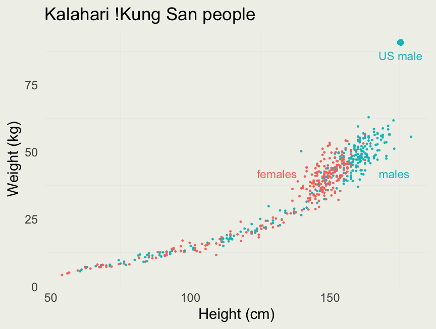
Deriving the model
- From McElreath’s Statistical Rethinking 2nd Ed., Ch 16
- The volume of the cylinder is: \(V = \pi r^2 h\)
- Assume width (\(2r\)) is proportional to the height \(h\): \(r = kh\)
- \(V = \pi r^2 h = \pi (kh)^2 h = \theta h^3\) where \(\theta\) absorbed other constant terms
- Assume weight is proportional to volume: \(w = kV\), \(w = k\theta h^3\)
- We will absorb \(k\) into \(\theta\), and so \(w = \theta h^3\)

Prior Predictive Simulation
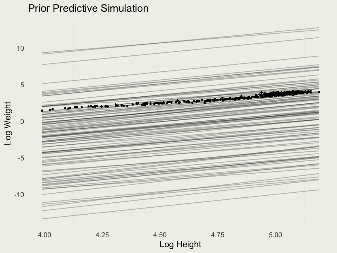
Prior Predictive Simulation
- We can examine what this looks like on the original scale by exponentiating the predictions:
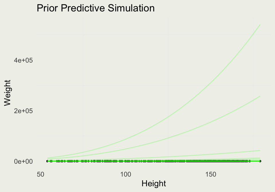
Prior Predictive Simulation
- Our intercept scale seems too wide, so we will make some adjustments:
m3 <- stan_glm(
  log_w ~ log_h,
  data = d,
  family = gaussian,
  prior = normal(3, 0.3),
  prior_aux = exponential(1),
  prior_intercept = normal(0, 2.5),
  prior_PD = 1,  # don't evaluate the likelihood
  seed = 1234,
  refresh = 0,
  chains = 4,
  iter = 600
)
d |>
  add_epred_draws(m3, ndraws = 100) |>
  ggplot(aes(y = weight, x = height)) +
  geom_point(size = 0.5) +
  geom_line(aes(y = exp(.epred), group = .draw),
            alpha = 0.25, color = 'green') +
  xlab("Height") + ylab("Weight") +
  ggtitle("Prior Predictive Simulation")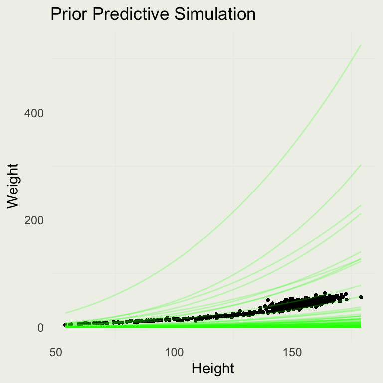
Comparing to the Linear Model
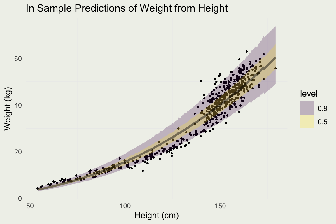
Plotting Prediction Intervals
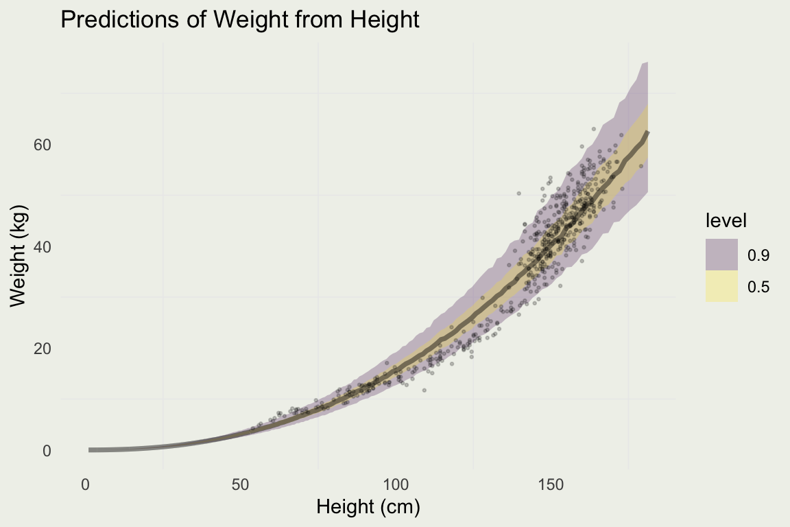
Predicting For New Data
log_h <- seq(0, 5.2, len = 500)
new_data <- tibble(log_h)
pred <- add_predicted_draws(new_data, m3)
pred |>
  ggplot(aes(x = exp(log_h), y = exp(.prediction))) +
  stat_lineribbon(.width = c(0.90, 0.50), alpha = 0.25) +
  xlab("Height (cm)") + ylab("Weight (kg)") + ggtitle("Predictions of Weight from Height") +
  geom_point(aes(y = weight, x = height), size = 0.5, alpha = 0.2, data = d)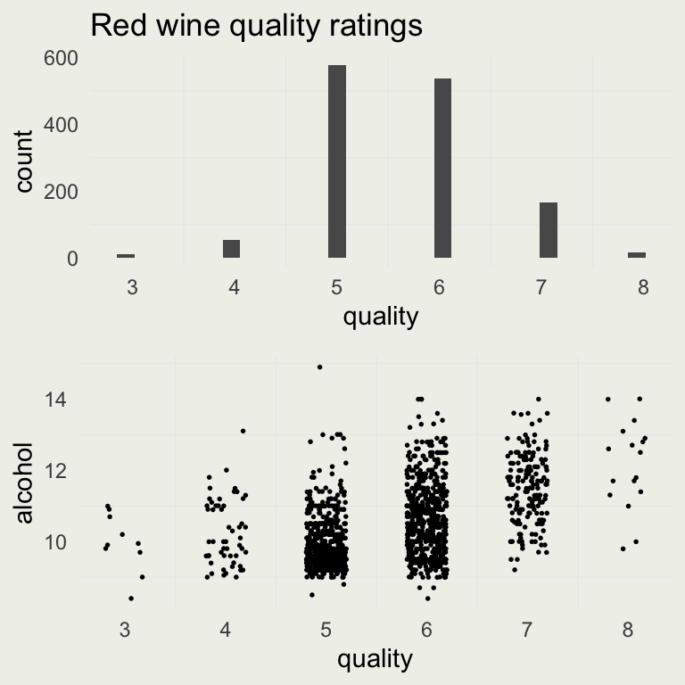
Example: Quality of Wine
- To build up a larger regression model, we will take a look at the quality of wine dataset from the UCI machine learning repository

Example: Quality of Wine
- Our task is to predict the (subjective) quality of wine from measurements like acidity, sugar, and chlorides
- The outcome is ordinal, which should be analyzed using ordinal regression, but we will start with linear regression
d <- readr::read_delim("data/winequality-red.csv")

# remove duplicates
d <- d[!duplicated(d), ]
p1 <- ggplot(aes(x = quality), data = d)
p1 <- p1 + geom_histogram() +
  ggtitle("Red wine quality ratings")
p2 <- ggplot(aes(quality, alcohol), data = d)
p2 <- p2 +
  geom_point(position =
               position_jitter(width = 0.2),
             size = 0.3)
grid.arrange(p1, p2, nrow = 2)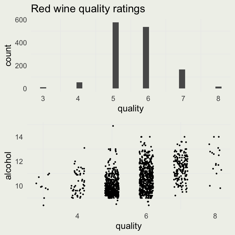
Example: Quality of Wine
- We can look at the inference using
mcmc_areas
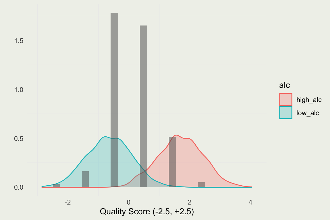
Example: Quality of Wine
- Let’s predict the rating at the high and low alcohol content
- On a standardized scale, that would correspond to an alcohol measurement of 4 and -2 (or about 8 and 15 on the original scale)
library(bayesplot)
d_new <- tibble(alcohol = c(-2, 4))
pred <- m1 |>
  posterior_predict(newdata = d_new) |>
  data.frame()
colnames(pred) <- c("low_alc", "high_alc")
pred <- tidyr::pivot_longer(pred, everything(),
                            names_to = "alc",
                            values_to = "value")
p <- ggplot(aes(x = value),
            data = pred)
p + geom_density(aes(fill = alc, color = alc),
                 alpha = 1/4) +
  geom_histogram(aes(x = quality,
                     y = after_stat(density)),
                 alpha = 1/2,
                 data = ds) +
  xlab("Quality Score (-2.5, +2.5)") + ylab("")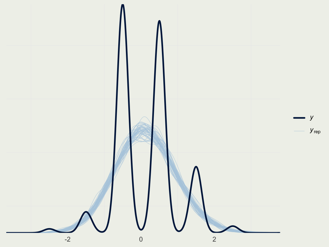
Example: Quality of Wine
- Naive way to show the posterior predictive check (don’t do this)
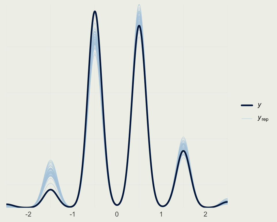
Example: Quality of Wine
- We can classify each prediction based on the distance to the nearest rating category
map_real_number <- function(x) {
  if (x < -2) {
    return(-2.5)
  } else if (x >= -2 && x < -1) {
    return(-1.5)
  } else if (x >= -1 && x < 0) {
    return(-0.5)
  } else if (x >= 0 && x < 1) {
    return(0.5)
  } else if (x >= 1 && x < 2) {
    return(1.5)
  } else if (x >= 2) {
    return(2.5)
  }
}
map_real_number <- Vectorize(map_real_number)
yrep_cat <- map_real_number(yrep1) |>
  matrix(nrow = nrow(yrep1), ncol = ncol(yrep1))
ppc_dens_overlay(ds$quality,
            yrep_cat[sample(nrow(yrep1), 50), ])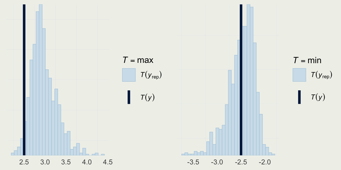
Example: Quality of Wine
- We can take a look at the distribution of a few statistics to check where the model is particularly strong or weak
Example: Quality of Wine
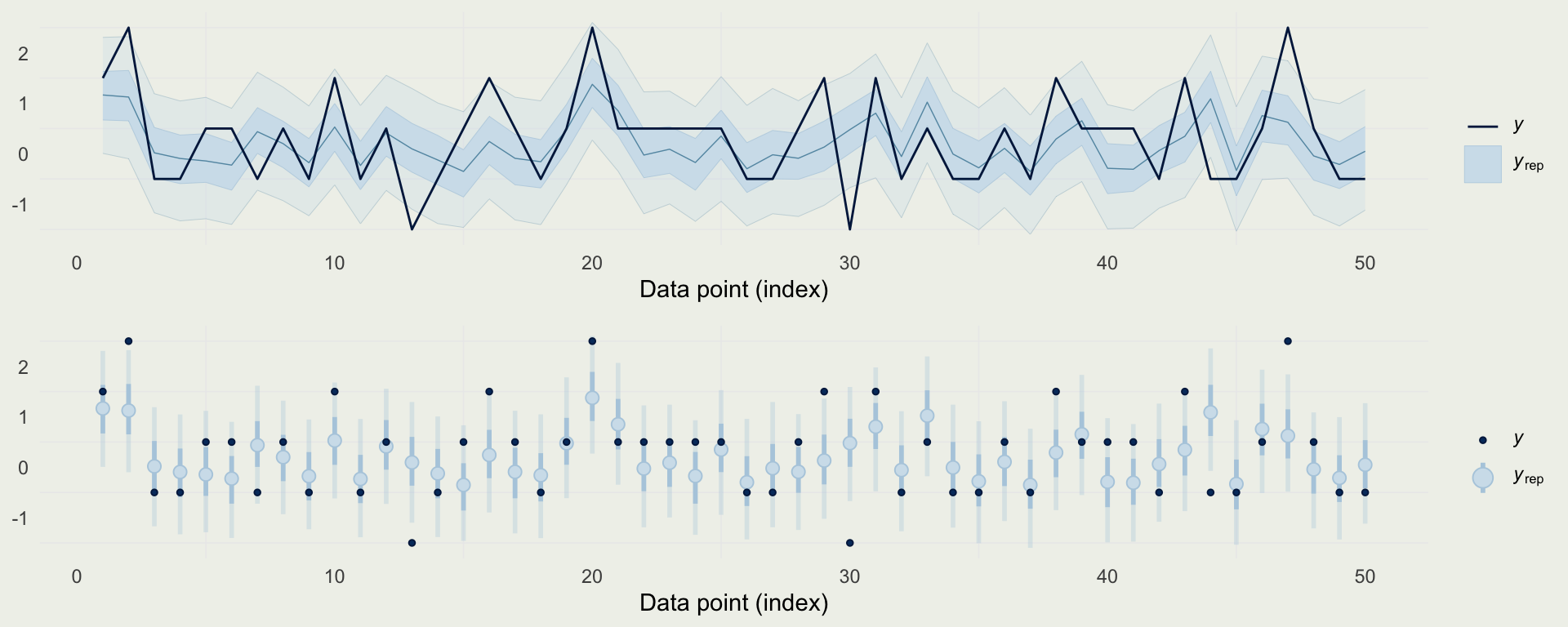
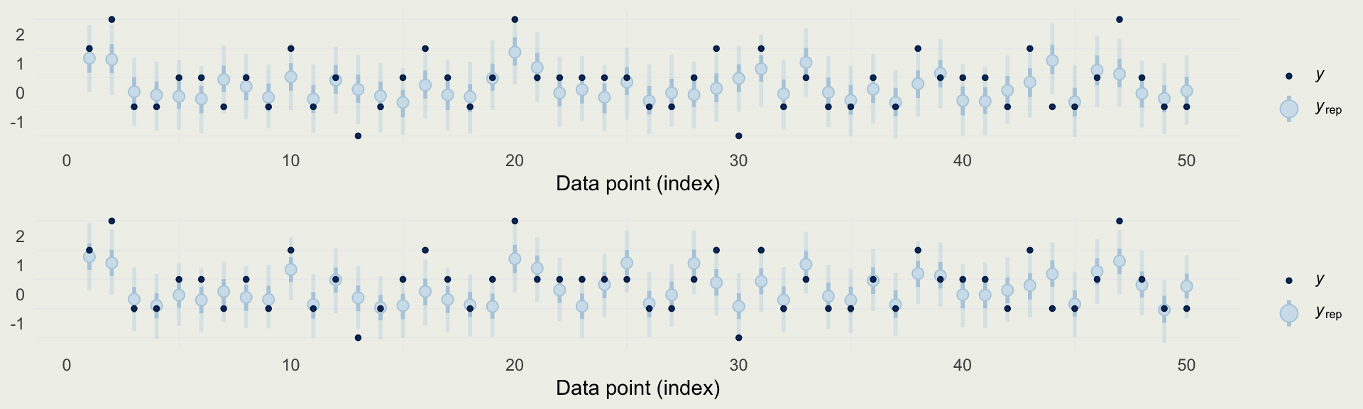
- We can also look at predictions directly, and compare them to observed data
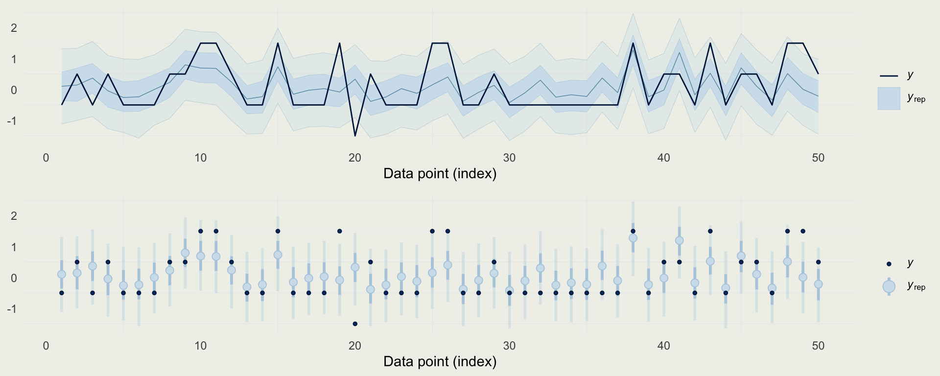
Example: Quality of Wine
- We can look at all the parameters in one plot, excluding
sigma
Example: Quality of Wine
- Did we improve the model?
- We will check accuracy using MSE for both models
- We will also check the width of posterior intervals
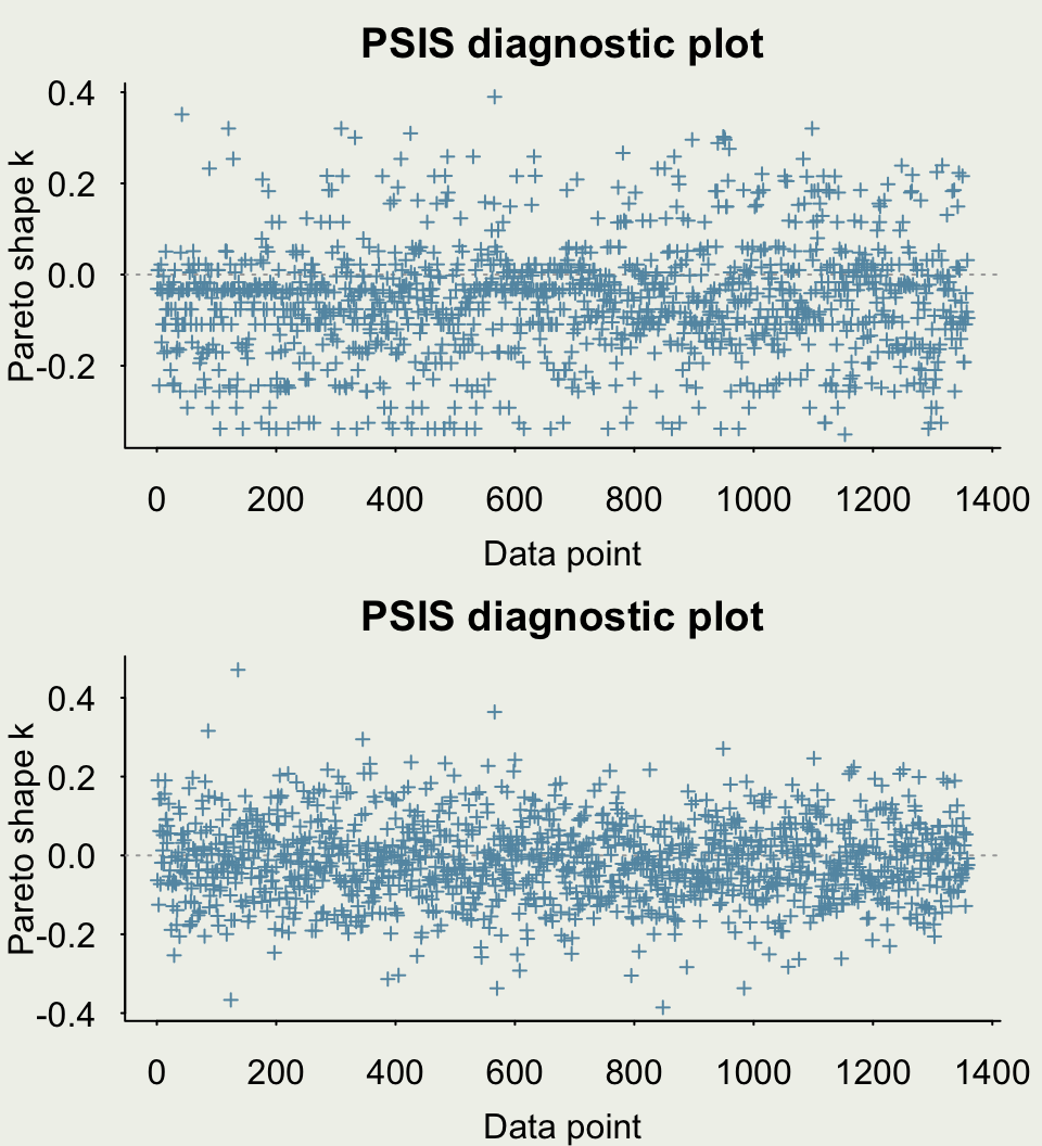
- Finally, we will compare the models using PSIS-LOO CV (preferred)
Example: Quality of Wine
- Let’s estimate PSIS-LOO CV, a measure of out-of-sample predictive performance
Poisson Simulation
- We can set up a forward simulation to generate Poisson data
- It’s a good practice to fit simulated data and see if you can recover the parameters from a known data-generating process
set.seed(123)
n <- 100
a <- 1.5
b <- 0.5
x <- runif(n, -5, 5)
eta <- a + x * b   # could be negative
lambda <- exp(eta) # always positive
y <- rpois(n, lambda)
sim <- tibble(y, x, lambda)
p <- ggplot(aes(x, y), data = sim)
p + geom_point(size = 0.5) +
  geom_line(aes(y = lambda),
            col = 'red',
            linewidth = 0.2) +
  ggtitle("Simulated Poisson Data")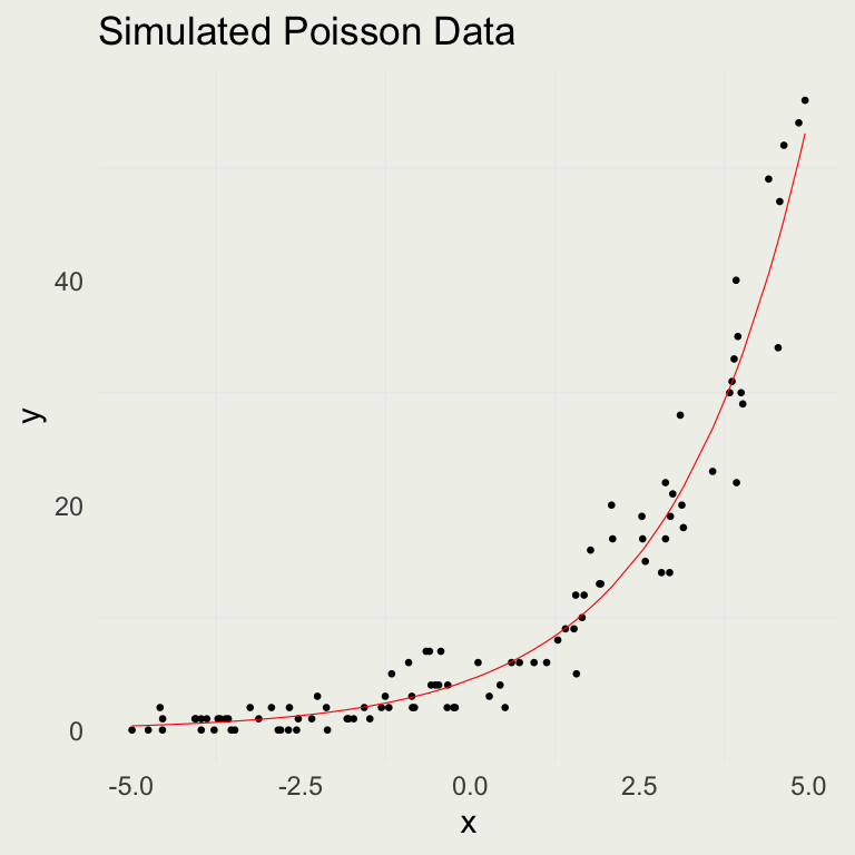
Checking Poisson Assumption
- We know that for Poisson model, \(\E(y_i) = \V(y_i)\), or equivalently \(\sqrt{\E(y_i)} = \text{sd}(y_i)\)
- We can check that the prediction errors follow this trend since we have a posterior predictive distribution at each \(y_i\)
library(latex2exp)
yrep <- posterior_predict(m3)
d <- tibble(y_mu_hat = sqrt(colMeans(yrep)),
            y_var = apply(yrep, 2, sd))
p <- ggplot(aes(y_mu_hat, y_var), data = d)
p + geom_point(size = 0.5) +
  geom_abline(slope = 1, intercept = 0,
              linewidth = 0.2) +
  xlab(TeX(r'($\sqrt{\widehat{E(y_i)}}$)')) +
  ylab(TeX(r'($\widehat{sd(y_i)}$)'))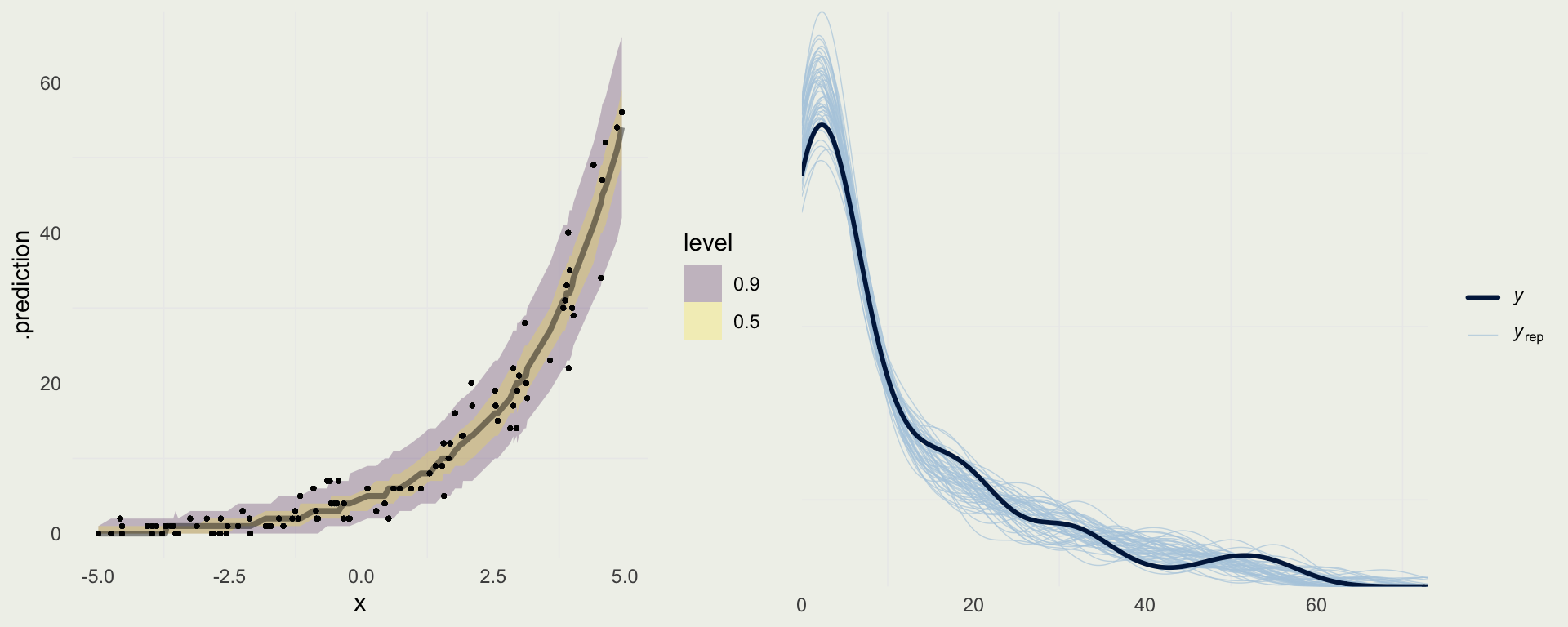
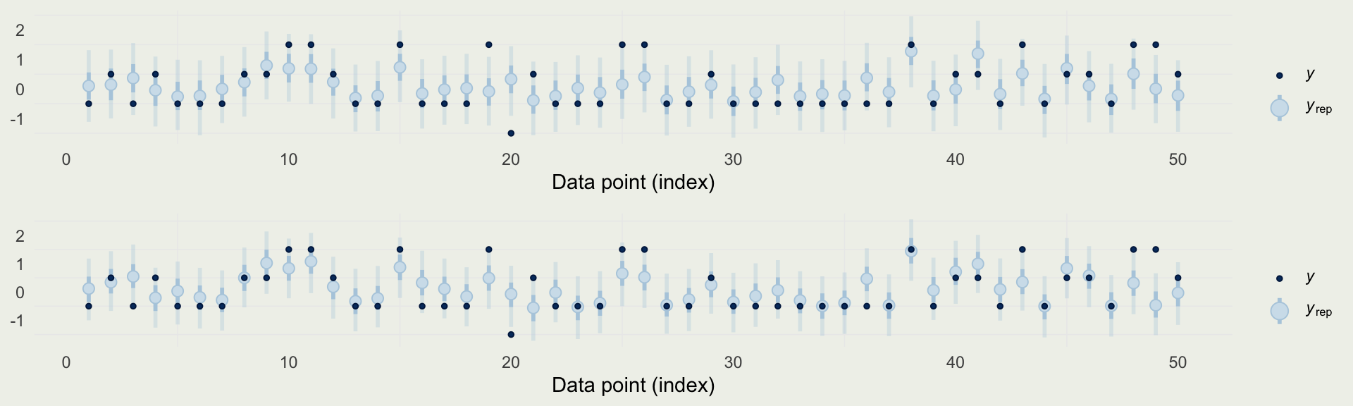
Posterior Predictive Checks
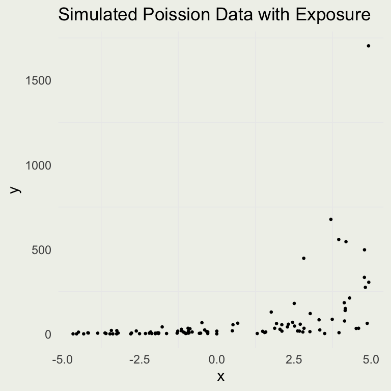
Adding Exposure
- Let’s check the effect of adding an exposure variable to the DGP
n <- 100
a <- 1.5
b <- 0.5
x <- runif(n, -5, 5)
u <- rexp(n, 0.2)
eta  <- a + x * b + log(u)
# or <- a + x * b

lambda <- exp(eta)
y <- rpois(n, lambda)
# or rpois(n, u * lambda)

sim_exposure <- tibble(y, x, lambda,
                       exposure = u)
p <- ggplot(aes(x, y), data = sim_exposure)
p + geom_point(size = 0.5) +
ggtitle("Simulated Poisson Data with Exposure")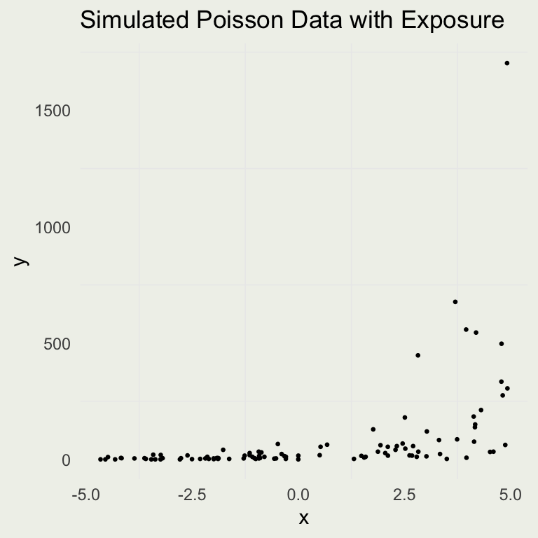
Checking Predictions
- Suppose we fit the model with and without the exposure term
m4 <- stan_glm(y ~ x,
               prior_intercept = normal(0, 1),
               prior = normal(0, 1),
               family = poisson(link = "log"),
               data = sim_exposure, refresh = 0,
               iter = 1200)
m5 <- stan_glm(y ~ x,
               prior_intercept = normal(0, 1),
               prior = normal(0, 1),
               family = poisson(link = "log"),
               offset = log(exposure),
               refresh = 0,
               data = sim_exposure, iter = 1200)
yrep_m4 <- posterior_predict(m4)
yrep_m5 <- posterior_predict(m5)
s <- sample(nrow(yrep_m4), 100)
p1 <- ppc_dens_overlay(log(sim_exposure$y + 1),
                       log(yrep_m4[s, ] + 1)) +
  ggtitle("No Exposure (log scale)")
p2 <- ppc_dens_overlay(log(sim_exposure$y + 1),
                       log(yrep_m5[s, ] + 1)) +
  ggtitle("With Exposure (log scale)")
pred4 <- add_predicted_draws(sim_exposure, m4)
pred5 <- add_predicted_draws(sim_exposure, m5,
offset = log(sim_exposure$exposure))
p3 <- pred4 |>
ggplot(aes(x = x, y = .prediction)) +
stat_lineribbon(.width = c(0.90, 0.50),
alpha = 0.25) +
geom_point(aes(x = x, y = y), size = 0.5,
alpha = 0.2)
p4 <- pred5 |>
ggplot(aes(x = x, y = .prediction)) +
stat_lineribbon(.width = c(0.90, 0.50),
alpha = 0.25) +
geom_point(aes(x = x, y = y), size = 0.5,
alpha = 0.2)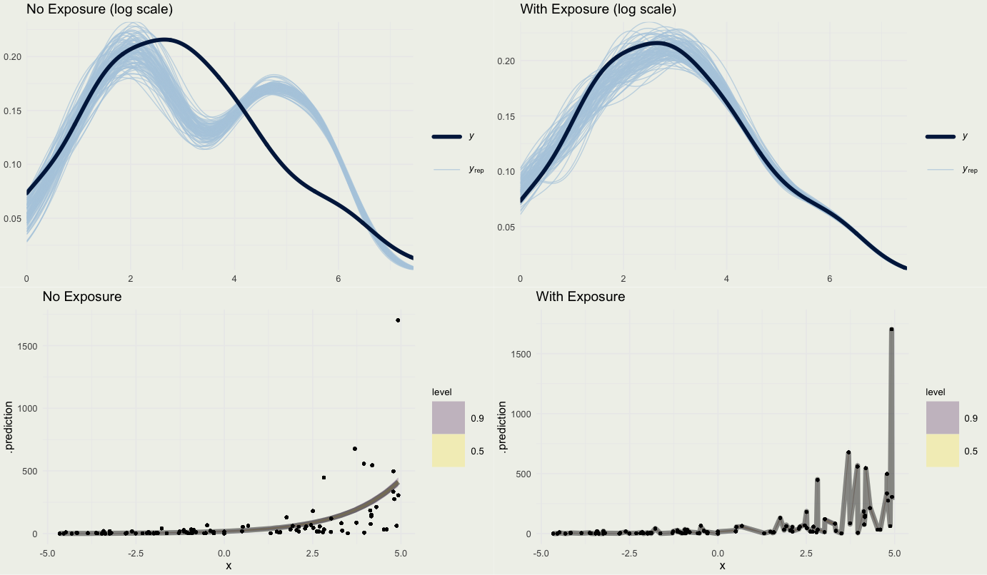
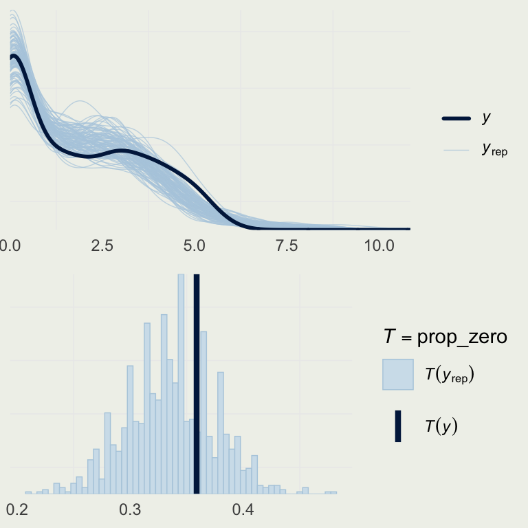
Example: Trapping Roaches
- How good is this model?
- Let’s look at the basic posterior predictive check
yrep_m7 <- posterior_predict(m7)
s <- sample(nrow(yrep_m7), 100)

# on the log scale,
# so we can better see the data
p1 <- ppc_dens_overlay(log(roaches$y + 1),
                 log(yrep_m7[s, ] + 1))

prop_zero <- function(y) mean(y == 0)
p2 <- pp_check(m7, plotfun = "stat",
               stat = "prop_zero",
               binwidth = .005)
grid.arrange(p1, p2, nrow = 2)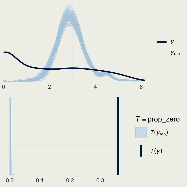
Example: Trapping Roaches
- How good is this model?
- Let’s look at the basic posterior predictive check
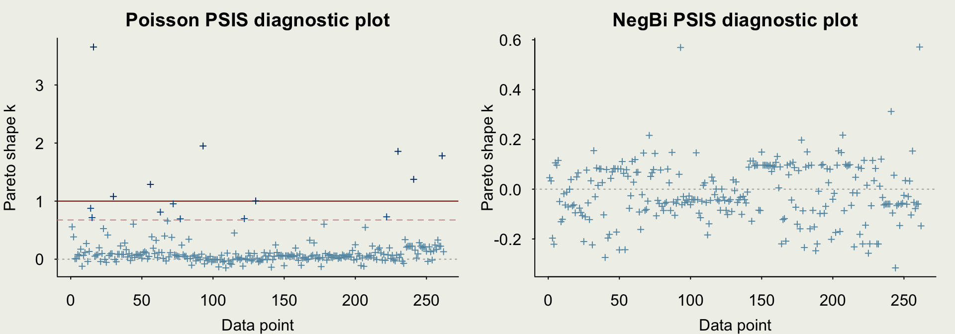
Example: Trapping Roaches
- Let’s check the comparison of the out-of-sample predictive performance relative to the Poisson model