[1] 0.1Bayesian Inference
NYU Applied Statistics for Social Science Research
Logistic Simulation
- As before, we can forward simulate data for logistic regression
- We will fit the data and try to recover the parameters
set.seed(123)
logit <- qlogis; invlogit <- plogis
n <- 100
a <- 1.2
b <- 0.4
x <- runif(n, -15, 10)
eta <- a + x * b
Pr <- invlogit(eta)
y <- rbinom(n, 1, Pr)
sim <- tibble(y, x, Pr)

p <- ggplot(aes(x, y), data = sim)
p <- p + geom_point(size = 0.5) +
  geom_line(aes(x, Pr), linewidth = 0.2) +
  geom_vline(xintercept = 0, color = "red", linewidth = 0.2,
             linetype = "dashed", alpha = 1/3) +
  geom_hline(yintercept = invlogit(a), color = "red", linewidth = 0.2,
             linetype = "dashed", alpha = 1/3) +
  geom_hline(yintercept = 0.50, linewidth = 0.2, linetype = "dashed", alpha = 1/3) +
  ggtitle(TeX("$y_i \\sim Bernoulli(logit^{-1}(1.2 + 0.4x_i))$")) +
  annotate("text", x = -5.5, y = invlogit(a) - 0.02,
           label = TeX("Intercept = $logit^{-1}(1.2)$ \\approx 0.77")) +
  annotate("text", x = -8, y = 0.53,
           label = TeX("$slope_{.5} = \\frac{0.4}{4} = 0.10$")) +
  ylab(TeX("$logit^{-1}(1.2 + 0.4x)$")); print(p)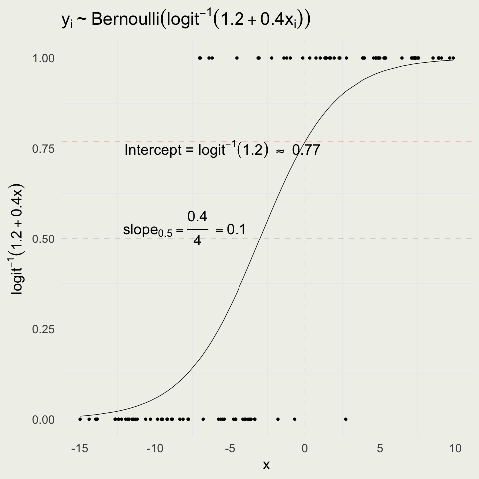
Interpreting Logistic Coefficients
- The intercept is the log odds of an event when \(x = 0\), \(\text{logit}^{-1}(1.2) = 0.77\)
- The slope changes depending on where you are on the curve
- When you are near 0.50, the slope of the inverse logit function (logistic curve) is 1/4 and so you can divide your coefficient by 4 to get a rough estimate
- This implies that if we go from \(x = -3\) to \(x = -2\), the probability will increase by about 0.10

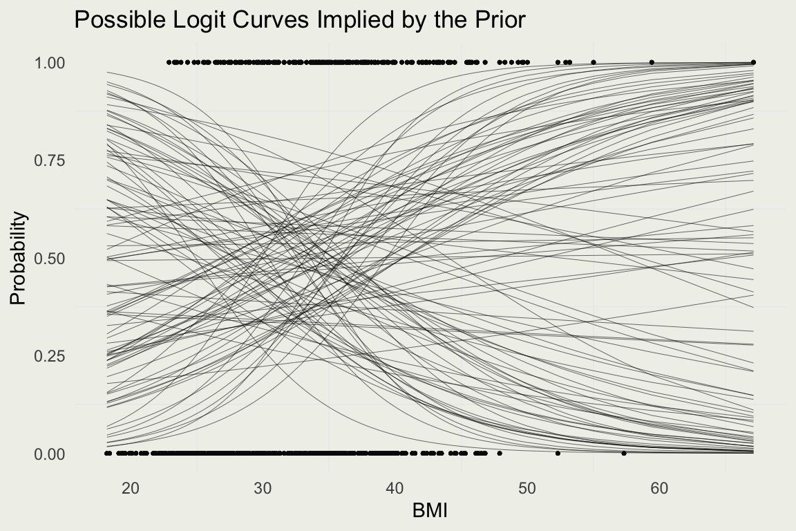
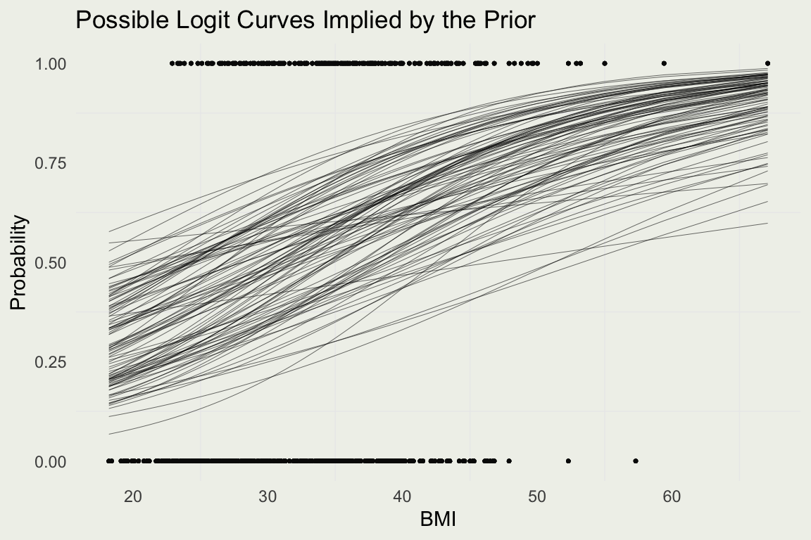
Generating Probability Data
- To get a sense of the variability in probability we can simulate from the prior distribution on the probability scale
prior_pred_logit <- function(x) {
  a <- rnorm(1, mean = 1.2, sd = 0.5)
  b <- rnorm(1, mean = 0.4, sd = 0.1)
  Pr <- invlogit(a + b * x)
  return(Pr)
}
prior_pred <- replicate(50, prior_pred_logit(x)) |>
  as.data.frame()

df_long <- prior_pred |>
  mutate(x = x) |>
  pivot_longer(cols = -x, names_to = "line", values_to = "y")

p <- ggplot(aes(x, y), data = df_long)
p + geom_line(aes(group = line), linewidth = 0.2, alpha = 1/5) +
  geom_line(aes(y = Pr), data = sim, linewidth = 0.5, color = 'red') +
  ylab(TeX("$logit^{-1}(\\alpha + \\beta x)$")) +
  ggtitle(TeX("Simulating from prior $logit^{-1}(\\alpha + \\beta x_i))$"),
  subtitle = TeX("$\\alpha \\sim Normal(1.2, 0.5)$ and $\\beta \\sim Normal(0.4, 0.1)$"))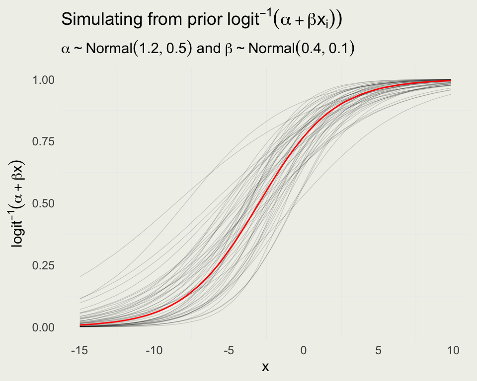
Two Truths and a Lie1
- One person tells three personal statements, one of which is a lie.
- Others discuss and guess which statement is the lie, and they jointly construct a numerical statement of their certainty in the guess (on a 0–10 scale).
- The storyteller reveals which was the lie.
- Enter the certainty number and the outcome (success or failure) and submit in the Google form. Rotate through everyone in your group so that each person plays the storyteller role once.
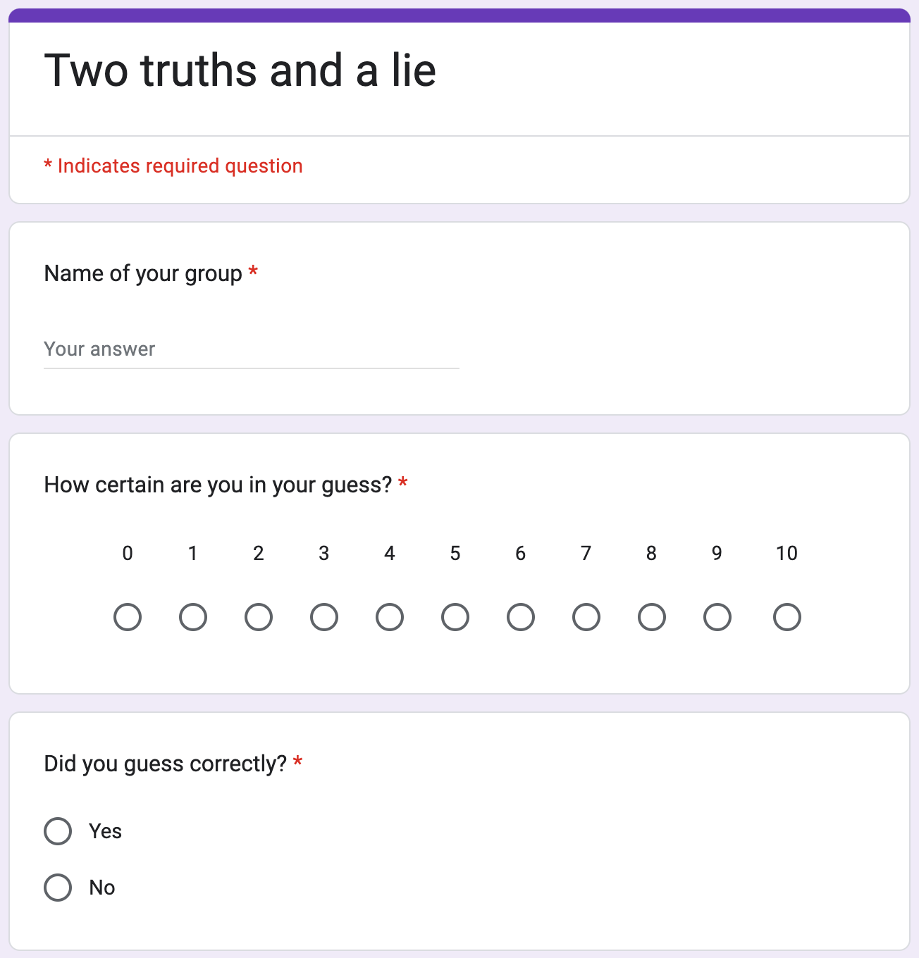
Two Truths and a Lie
https://tinyurl.com/two-truths-and

Example: Diabetes
- It is well-known that people with high BMI are at risk for Type 2 diabetes
- We can do some exploratory analysis to check this
p1 <- ggplot(pima, aes(x = mass)) +
  geom_density(aes(group = diabetes, fill = diabetes, color = diabetes), alpha = 1/5) +
  xlab("BMI")
p2 <- pima |>
  drop_na() |>
  mutate(bmi_cut = cut(mass, breaks = seq(15, 70, by = 5))) |>
  group_by(bmi_cut) |>
  summarize(p = mean(diabetes == "pos"),
            n = n(),
            se = sqrt(p * (1 - p) / n),
            lower = p - se,
            upper = p + se) |>
  ggplot(aes(x = bmi_cut, y = p)) +
  geom_point() + geom_linerange(aes(ymin = lower, ymax = upper), linewidth = 0.2) +
  xlab("BMI range") + ylab("Proportion") +
  ggtitle("Proportion of diabetics by BMI +/- 1 SE")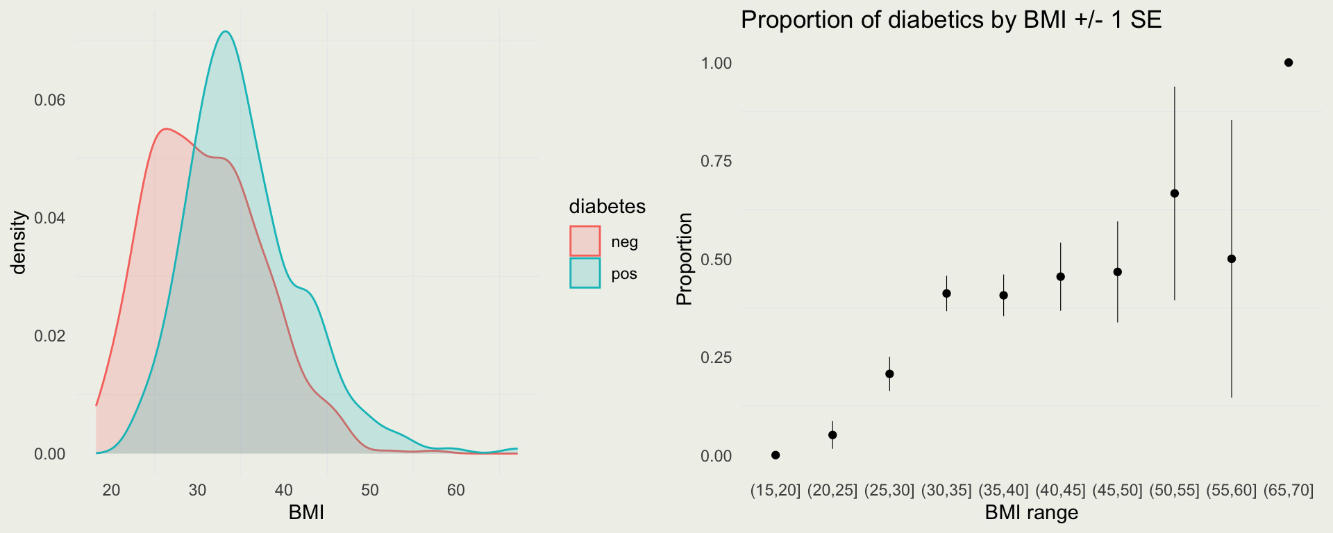
Example: Diabetes
Example: Diabetes
Example: Diabetes
- There are no sampling problems, but we should still check the diagnostics
Example: Diabetes
- We can examine the posterior probability of diabetes among this population (women who were at least 21 years old, and of Pima Indian heritage)
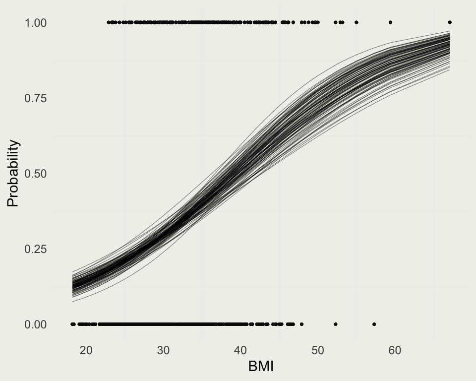
Example: Diabetes
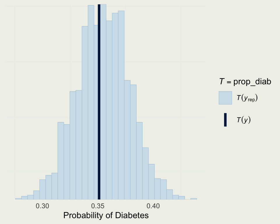
- We can also see the posterior predictive distribution of the probability of diabetes
ShinyStan Demo
- To install, run
install.packages("shinystan"), then launch withlaunch_shinystan(m3)

Example: Diabetes
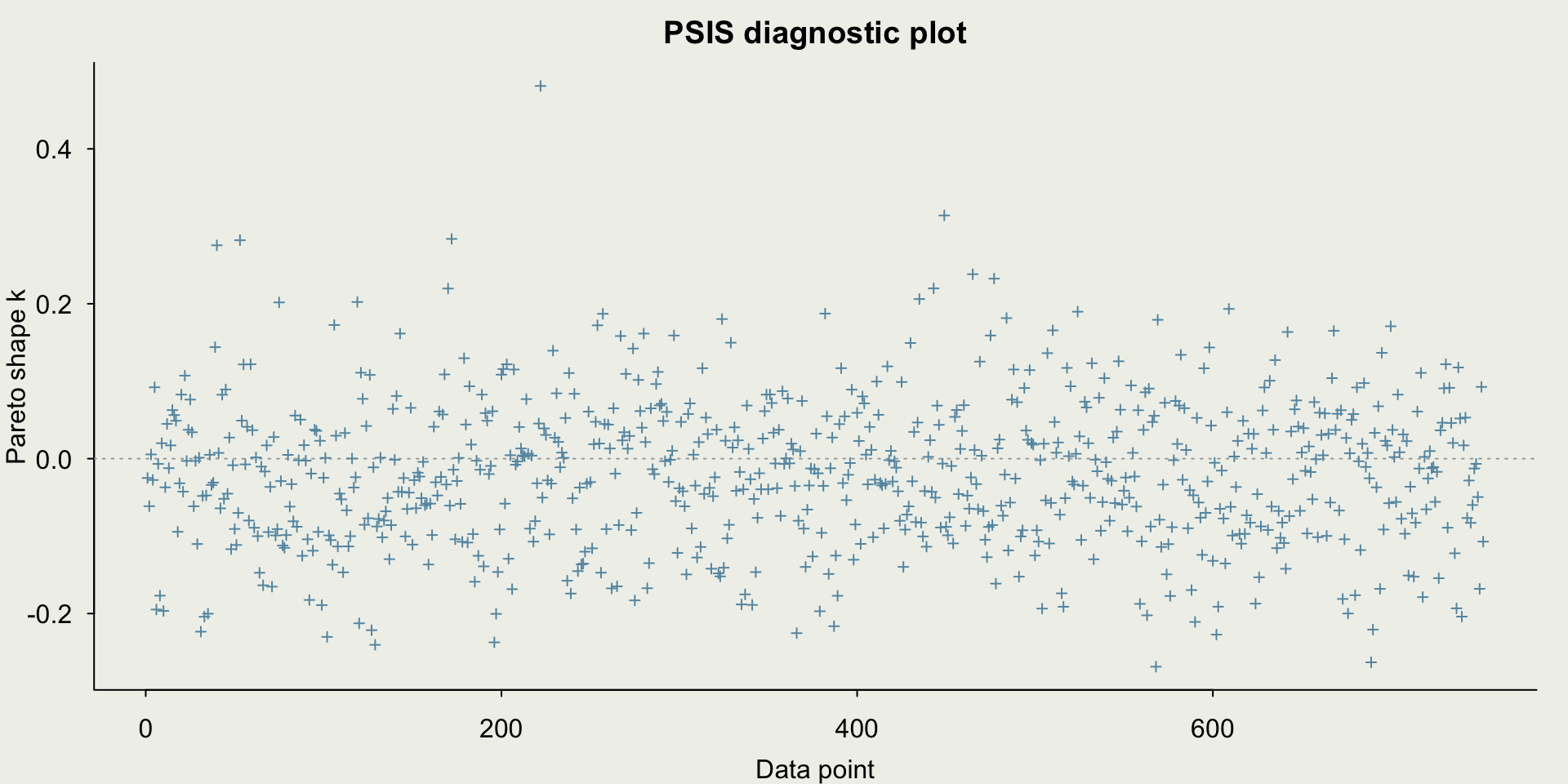
- We can perform model comparison using several methods
- One way is to assess classification accuracy under different probability cut points, which is often done in Machine Learning (ROC/AUC)
- A better way is to use LOO (
looandloo_comparein R)
Introduction to Hierarchical Models
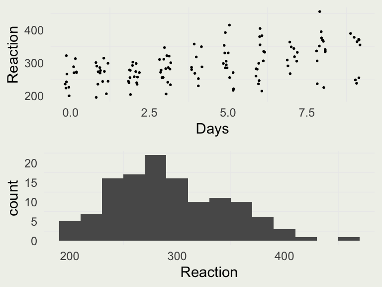
Sleep Data
- Let’s look at a classic dataset called
sleepstudyfromlme4package - These data are from the study described in Belenky et al. (2003), for the most sleep-deprived group (3 hours time-in-bed) and for the first 10 days of the study, up to the recovery period
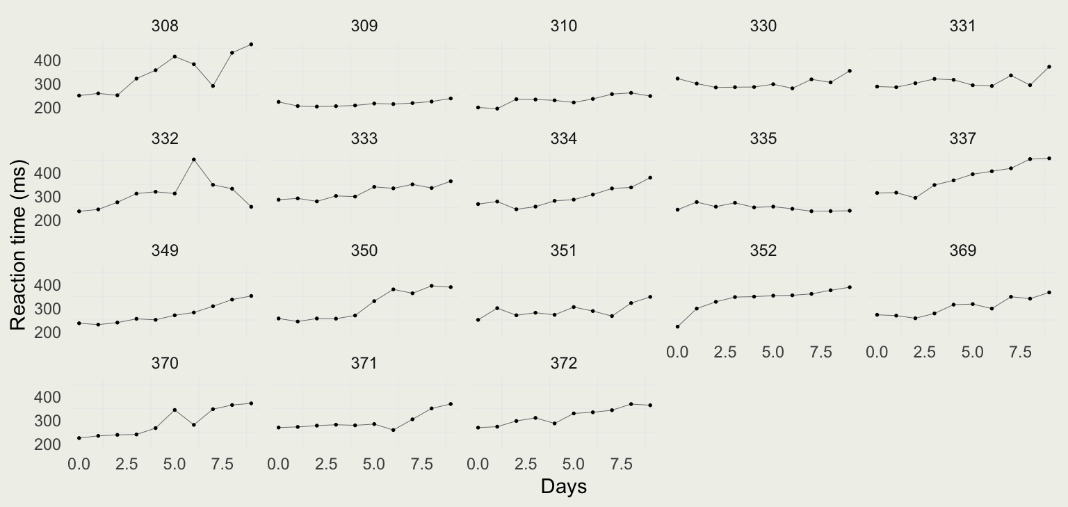
Sleep Data
- To get a better sense of the differences in per-Subject reaction time distributions, we can plot them side by side
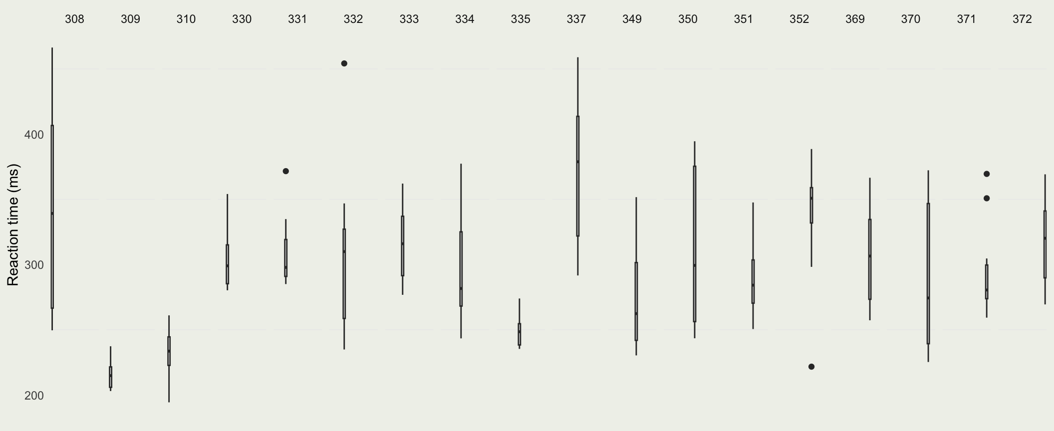
Pooling
- Pooling has to do with how much regularization we induce on parameter estimates in each cluster; sometimes this is called shrinkage
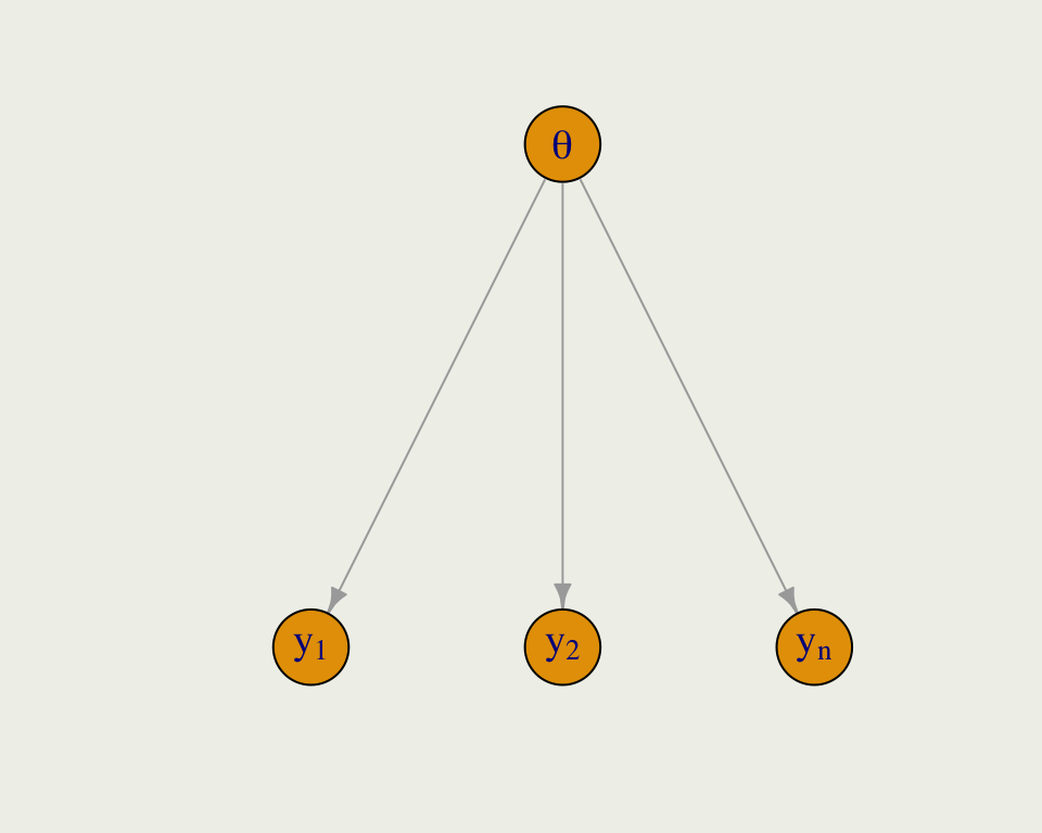
- Complete pooling ignores the clusters and estimates a global parameter
- Even though reaction time \(y_i\), belongs to subject \(j\), we ignore the groups and index all the \(y\)s together
Pooling
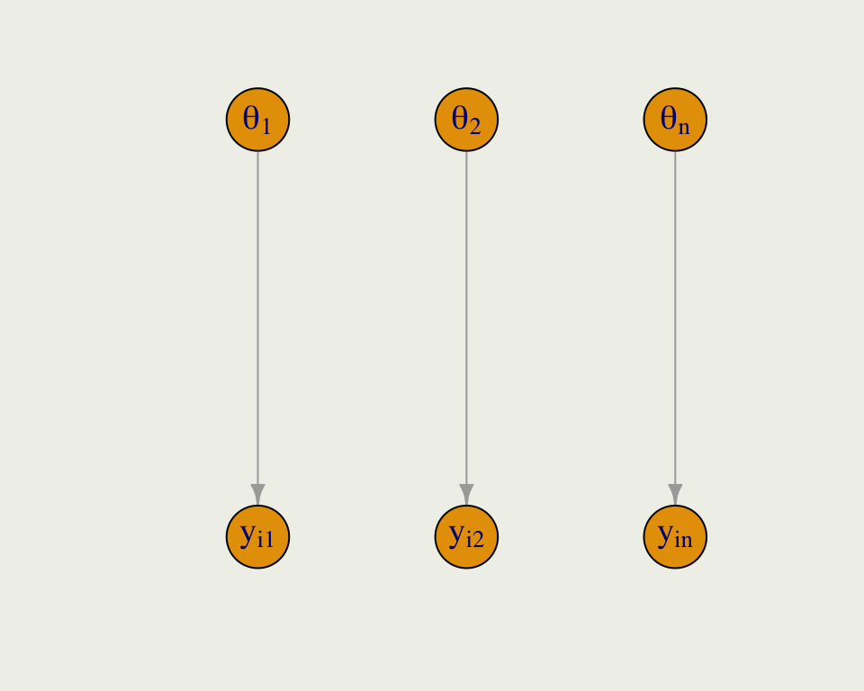
- Complete pooling is the opposite of no pooling, where we estimate a separate model for each group
- Here, we have \(n\) subjects, and \(y_{ij}\) refers to the \(i\)th reaction time in subject \(j\)
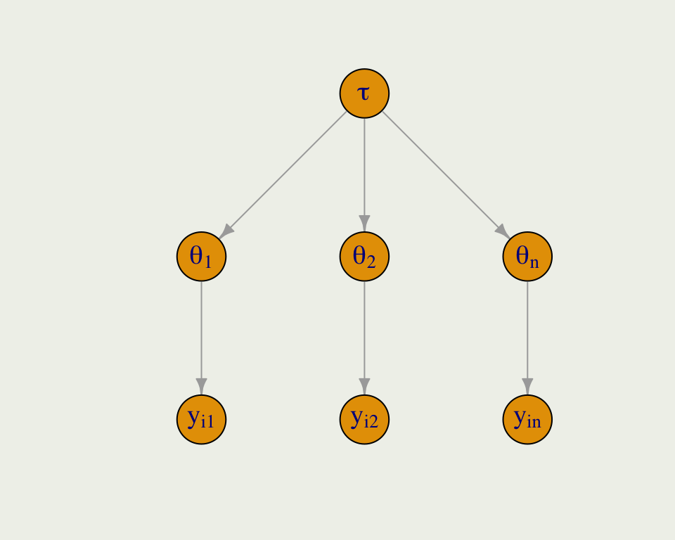
Partial Pooling
- Partial pooling is the compromise between the two extremes
- Like any other parameter in a Bayesian model, the global hyperparameter \(\tau\) is given a prior and is learned from the data
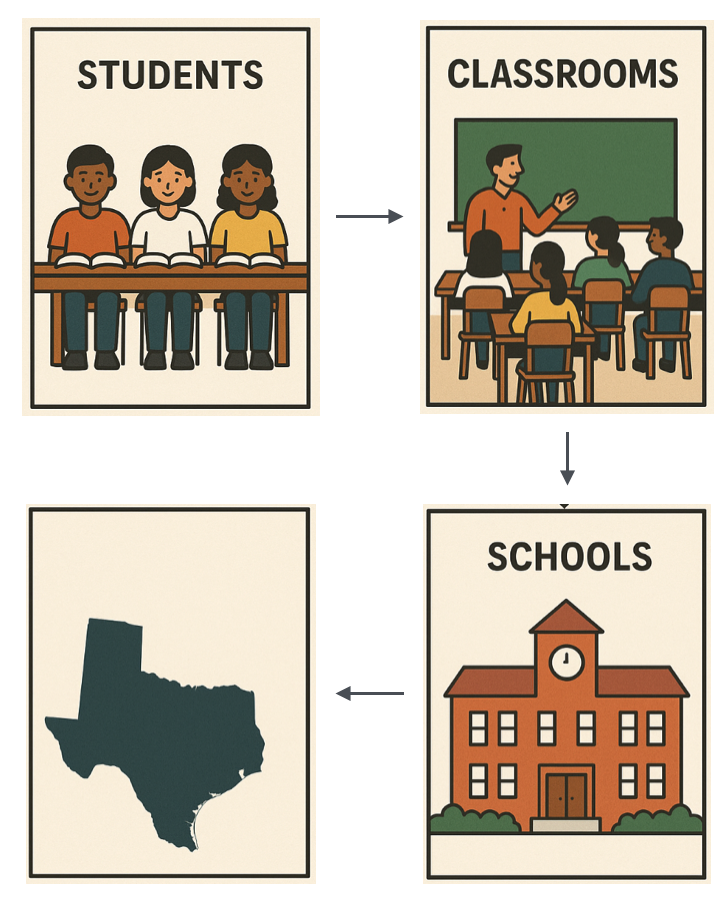
- There could be multiple levels of nesting, say students within schools, within states, etc.
Sleep Data
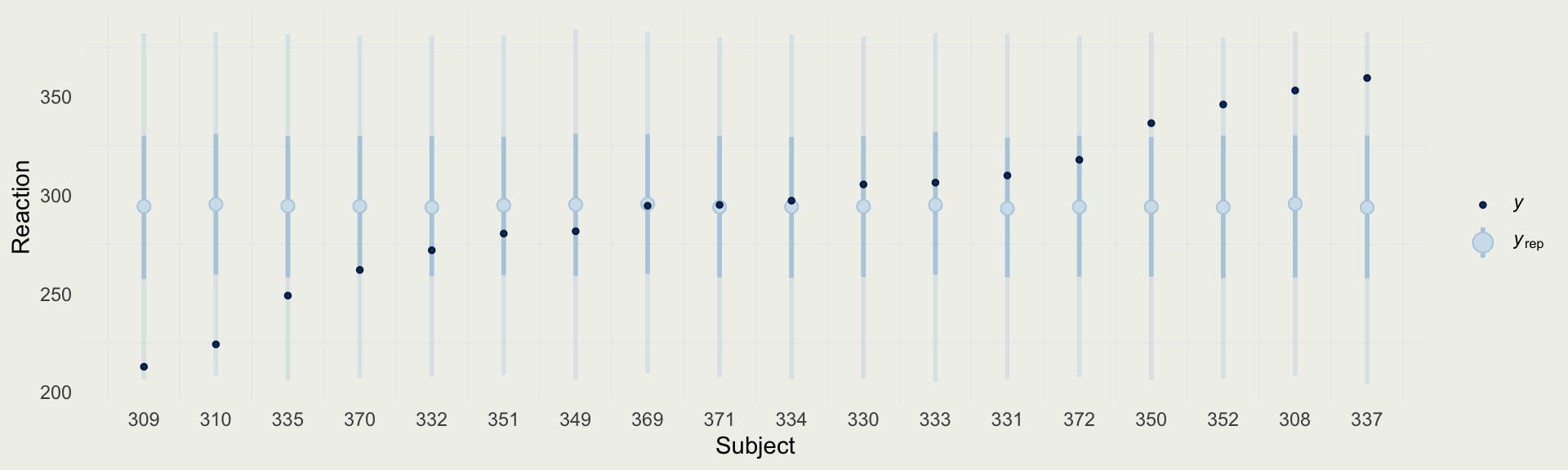
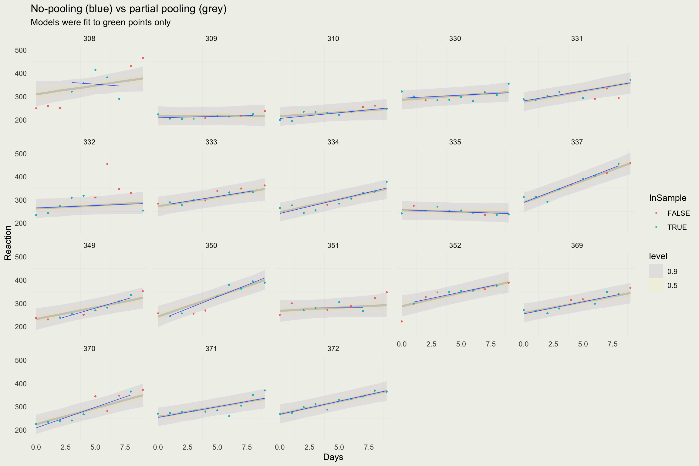
- Let’s build three models for the sleep data, starting with complete pooling, which is what we have been doing all along
- We will start with the intercept-only model
- These data contain the same number of observations per Subject, which is unusual, so we will make it more realistic by removing 30% of the measurements
Sleep Data
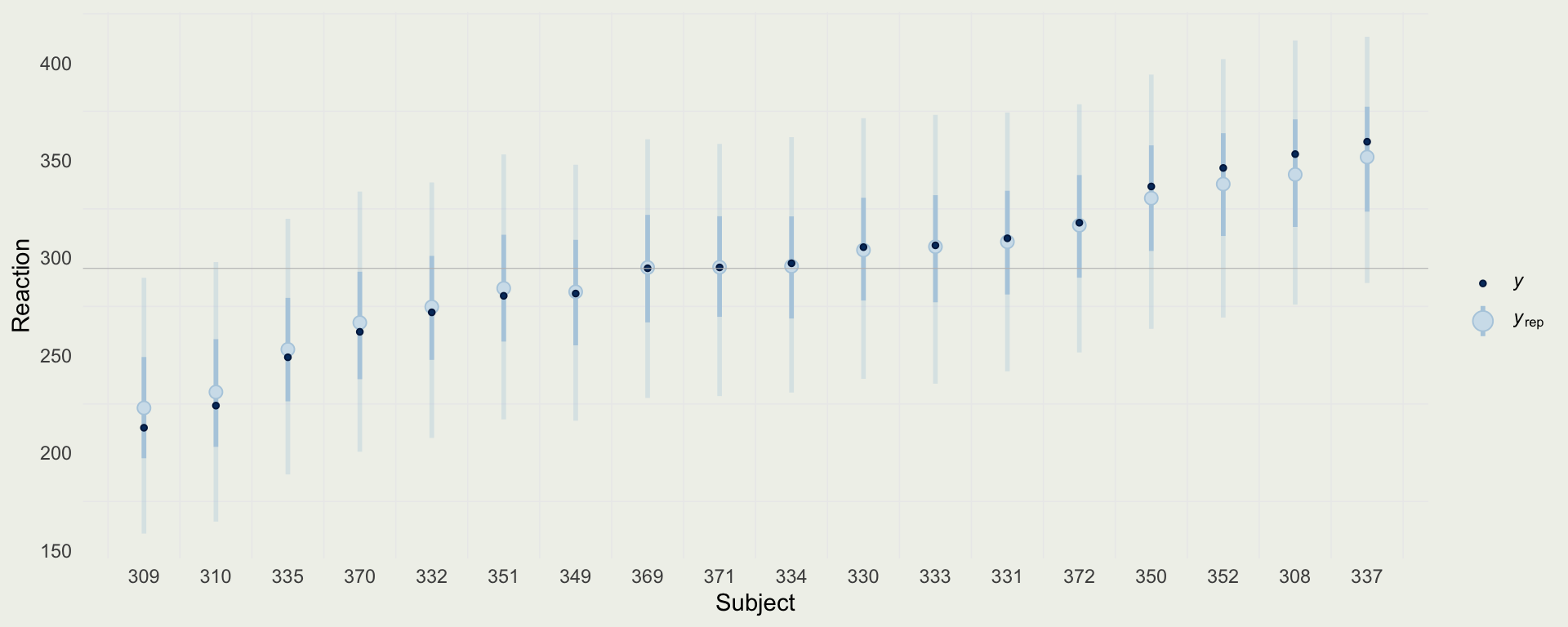
- We can compare the predictions from the complete-pooling model to the reaction times of each subject
Sleep Data
- We can compare the predictions from the no-pooling model to the reaction times of each subject
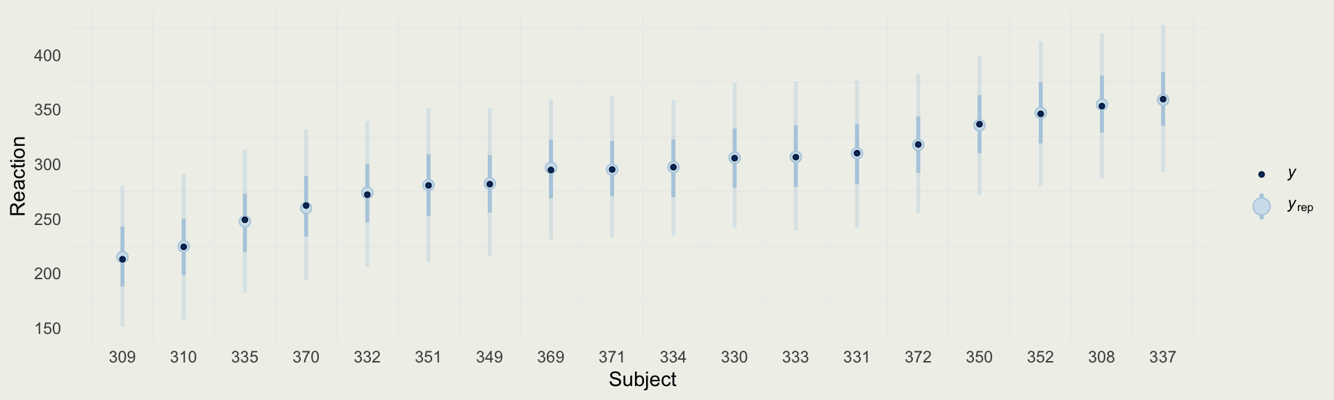
- What are some of the limitations of this approach?
Building a Hierarchical Model
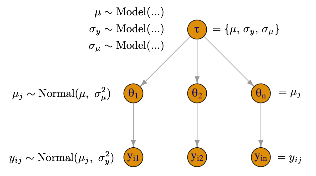
- \(\mu_j\) is an average reaction time for subject \(j\)
- \(\sigma_y\) is the within-subject variability of reaction times
- \(\mu\) is the global average of reaction times across all subject
- \(\sigma_{\mu}\) is subject to subject variability of reaction times
- Top-level parameters get fixed priors and induce the degree of pooling
Computing \(\mu_j\)
# A tibble: 6 × 7
  Subject      mu_j .lower .upper .width .point .interval
  <chr>       <dbl>  <dbl>  <dbl>  <dbl> <chr>  <chr>
1 Subject:308  344.   318.   369.    0.9 mean   qi
2 Subject:309  223.   200.   245.    0.9 mean   qi
3 Subject:310  231.   211.   252.    0.9 mean   qi
4 Subject:330  304.   285.   324.    0.9 mean   qi
5 Subject:331  308.   284.   330.    0.9 mean   qi
6 Subject:332 275. 252. 298. 0.9 mean qi 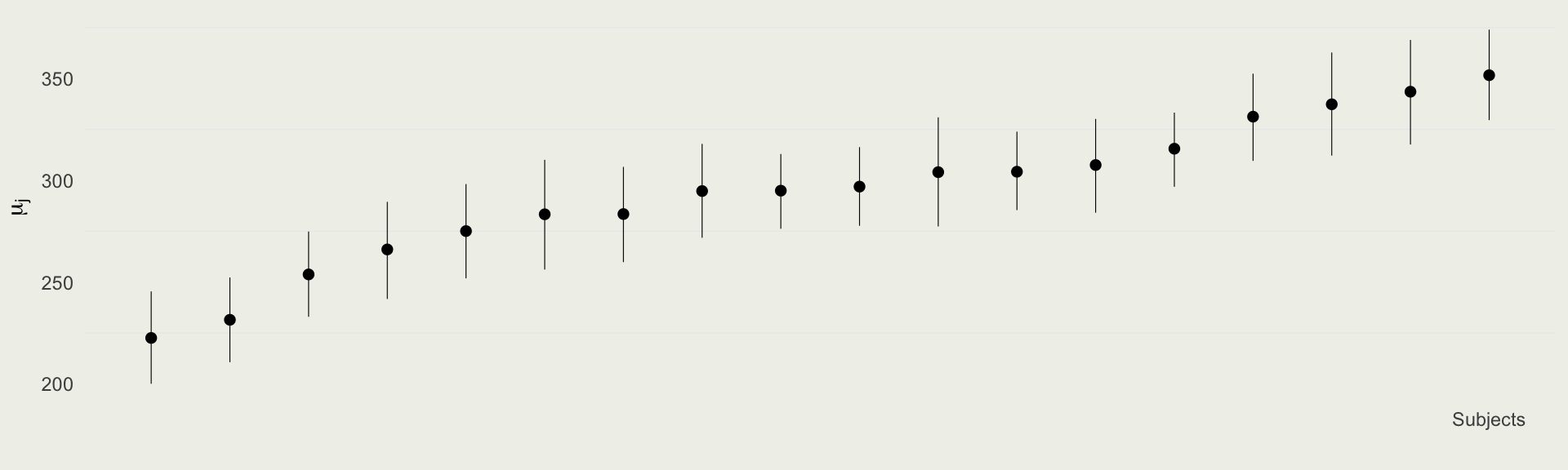
Sleep Data
- We can see the effects of hierarchical pooling below
- Subjects that are farther away from \(\E(\mu) = 294\)(ms) and the ones that have fewer observations are pooled more towards the global mean
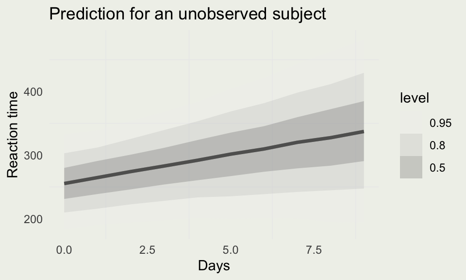
Predicting for a New Subject
- We saw that we can make predictions for reaction times of subjects that were part of the model
- But we can also make predictions for unobserved subjects by drawing from the “population” distribution, as opposed to subject-specific parameters
new_subj <- data.frame(Days = 0:9,
              Subject = as.factor(rep(400, 10)))
ypred_subj <- posterior_predict(m4,
                        newdata = new_subj)
new_subj |>
  add_predicted_draws(m4) |>
  ggplot(aes(x = Days)) +
  stat_lineribbon(aes(y = .prediction),
                  .width = c(.9, .8, .5),
                  alpha = 0.25) +
  ylab("Reaction time") +
  ggtitle("Prediction for an unobserved subject") +
  scale_fill_brewer(palette = "Greys")