| year | group | score | correct |
|---|---|---|---|
| Y2026 | Bayesian In-Friends | 6 | 1 |
| Y2026 | Bayesian in-friends | 4 | 0 |
| Y2026 | City girls | 4 | 0 |
| Y2026 | The jersey boys | 4 | 1 |
| Y2026 | the jersey boys | 4 | 0 |
| Y2026 | Bayesian in-friends | 5 | 1 |
| Y2026 | City girls | 5 | 0 |
| Y2026 | the jersey boys | 8 | 0 |
| Y2026 | City girls | 7 | 0 |
| Y2026 | city girls | 7 | 0 |
Two Truths and a Lie
Certainty and Accuracy in Guessing
Introduction
This activity was designed by Andrew Gelman and originally published in:
Gelman, A. (2023). “Two Truths and a Lie” as a class-participation activity. The American Statistician, 77(1), 97–101.
Data Used
This analysis uses the Google Sheet tabs selected by data_mode = "both". The current-year tab is Y2026; the previous available tab in the workbook is Y2024. The response variable is whether the group guessed the lie correctly, coded as 1 for a correct guess and 0 for an incorrect guess. The predictor is the group’s certainty score on a 0 to 10 scale.
The table shows the cleaned observations used in the model. Rows with missing certainty scores or missing outcomes are removed before fitting the model. The year column identifies which worksheet each response came from, which matters when current and previous data are combined.
| year | responses | mean_score | accuracy |
|---|---|---|---|
| Y2024 | 29 | 5.86 | 0.41 |
| Y2026 | 10 | 5.40 | 0.30 |
This summary gives a quick check on the sample size, average certainty, and observed accuracy. The accuracy column is the raw proportion of correct guesses before fitting any model.
Certainty and Correct Guesses
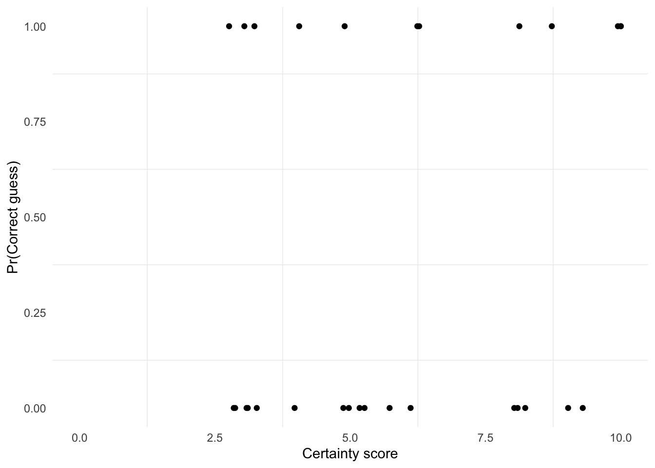
Each point is one group’s guess. The horizontal position is the certainty score, with slight jitter added only to reduce overplotting. The vertical position is the outcome: 1 means the group guessed correctly and 0 means it did not. If both years are selected, point color identifies the worksheet year.
Bayesian Logistic Regression
Let \(y_i\) indicate whether guess \(i\) was correct, and let \(x_i\) be the certainty score for that guess. We model the probability of a correct guess with a logistic regression:
\[ \begin{aligned} y_i &\sim \textrm{Bernoulli}(p_i) \\ \textrm{logit}(p_i) &= \alpha + \beta x_i \\ p_i &= \textrm{logit}^{-1}(\alpha + \beta x_i). \end{aligned} \]
The intercept \(\alpha\) is the log odds of a correct guess when the certainty score is 0. Because the game has two truths and one lie, random guessing has probability \(1/3\) of identifying the lie. That implies a natural prior center for the intercept:
\[ \textrm{logit}(1/3) = \log\left(\frac{1/3}{2/3}\right) \approx -0.69. \]
For the slope, \(\beta\) is the change in log odds for a one-point increase in certainty. On the odds scale, a one-point increase multiplies the odds of a correct guess by \(\exp(\beta)\). If \(\beta = 0\), then \(\exp(0) = 1\), meaning certainty has no association with accuracy. If \(\beta = 1\), then \(\exp(1) \approx 2.7\), meaning each one-point increase in certainty nearly triples the odds of a correct guess, which is already a large effect on a 0 to 10 scale. So a weakly informative prior centered at 0 with scale 0.5 is reasonable, even though one might expect the effect to be more likely positive than negative.
The model uses the following priors:
\[ \begin{aligned} \alpha &\sim \textrm{Normal}(\textrm{logit}(1/3), 1) \\ \beta &\sim \textrm{Normal}(0, 0.5). \end{aligned} \]
fit <- stan_glm(
  correct ~ score,
  prior_intercept = normal(qlogis(1 / 3), 1),
  prior = normal(0, 0.5),
  family = binomial(link = "logit"),
  data = data,
  iter = 500,
  refresh = 0,
  seed = 123
)
print(fit, digits = 2)
stan_glm
family: binomial [logit]
formula: correct ~ score
observations: 39
predictors: 2
------
Median MAD_SD
(Intercept) -1.20 0.82
score 0.12 0.14
------
* For help interpreting the printed output see ?print.stanreg
* For info on the priors used see ?prior_summary.stanregThe fitted output reports posterior summaries for \(\alpha\) and \(\beta\). The intercept describes baseline guessing performance at certainty score 0, while the slope describes how the odds of a correct guess change as certainty increases. Positive posterior mass for \(\beta\) supports the idea that more confident guesses tend to be more accurate.
Fitted Relationship
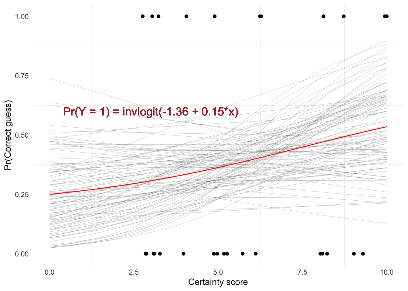
The thin gray curves are 100 draws from the posterior distribution, so they show uncertainty about the fitted relationship. The red line is the posterior mean relationship. When the gray lines are widely spread apart, the data leave more uncertainty about the probability of a correct guess at that certainty score.
Using the posterior mean coefficients, the estimated probability of a correct guess is about 0.23 at certainty score 0 and about 0.5 at certainty score 10. This comparison summarizes the fitted change across the observed certainty scale.
We can also compute posterior predictive summaries for specific certainty scores. Here the values are expected probabilities of a correct guess for someone with certainty scores 0, 5, and 10.
| Certainty score | 5% | 50% | 95% |
|---|---|---|---|
| 0 | 0.06 | 0.23 | 0.57 |
| 5 | 0.23 | 0.35 | 0.50 |
| 10 | 0.24 | 0.49 | 0.76 |
The median column is the posterior median probability at each certainty score. The 5% and 95% columns give a central 90% posterior interval for the expected probability, showing how uncertain the fitted model is at each point on the certainty scale.
Wider Score Range
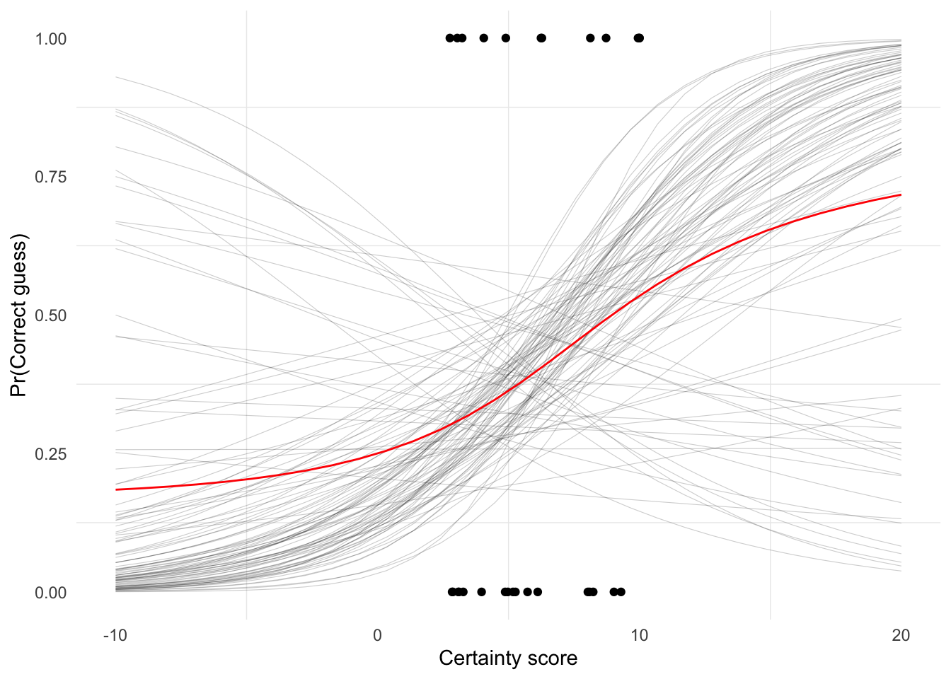
This plot extends the fitted logistic curve beyond the actual 0 to 10 certainty scale. It is useful for seeing the full S-shape implied by the logistic model, but values below 0 or above 10 are extrapolations rather than possible certainty scores from the activity.