SMaC: Statistics, Math, and Computing

APSTA-GE 2006: Applied Statistics for Social Science Research

Eric.Novik@nyu.edu | Summer 2025 | Session 1

Course Objectives

• This course will help you to prepare for the A3SR MS Program by covering the minimal necessary foundation in computing, math, and probability.

• After completing the course, you will be able to write simple R programs and perform simulations, plot and manipulate data, solve basic probability problems, and understand the concept of regression

\[ \DeclareMathOperator{\E}{\mathbb{E}} \DeclareMathOperator{\P}{\mathbb{P}} \DeclareMathOperator{\V}{\mathbb{V}} \DeclareMathOperator{\L}{\mathscr{L}} \DeclareMathOperator{\I}{\text{I}} \]

Course Format

• The course will run for two weeks, five days per week, 3 hours per day

• Each day will consist of:

  • ~30-minute going over the homework questions

  • ~1.5-hour lecture

  • ~1-hour hands of exercises

• The course will be computationally intensive – we will write many small programs.

Course Outline

• Introduction to the R language, RStudio, and R Markdown.

• Basic differentiation. Meaning of the derivative. Numeric and symbolic differentiation and optimization.

• Basic integration. Riemann integral and basic rules of integration.

• Review of one-dimensional probability. Conditional probability, random variables, and expectations. Solving probability problems by simulation.

• Discrete distributions like Bernoulli and Binomial and continuous distributions like Normal and Exponential

• Introduction to Linear Algebra. Vectors and vector arithmetic. Matrixes and matrix operations.

• Manipulating and graphing data and Exploratory Data Analysis

• Programming basics: variables, flow control, loops, functions, and writing simulations

• Introduction to basic statistical inference and linear regression.

References

• Hands-On Programming with R, Grolemund (2014)

• R for Data Science 2e, Wickham et al. (2023)

• Calculus Made Easy, Thompson (1980)

• Calculus, Herman et al. (2016)

• YouTube: Essence of Calculus, Sanderson (2018a)

• Optional: YouTube: Essense of Linear Algebra, Sanderson (2018b)

• Optional: Introduction to Linear Algebra, Boyd and Vandenberghe (2018)

• Optional: Matrix Cookbook, Petersen and Pedersen (2012)

• Intoduction to Probability, Blitzstein and Hwang (2019)

Where are you from?

Session 1 Outline

• The big picture – costs and benefits

• Setting up an analysis environment

• RStudio projects

• Working with interpreted languages like R

• Some basic R syntax and elements of R style

• Generating data with R

• Some basic R and ggplot graphics

• Writing your first Monte Carlo simulation

Some Mistakes Are Silly

Some Mistakes Are Deadly

On January 28, 1986, shortly after launch, Shuttle Challenger exploded, killing all seven crew members.

• O-Ring Data
• Binomial Model
• References

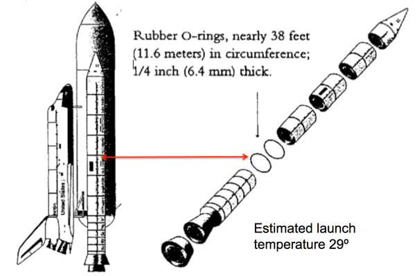
• Probability of 1 or more rings being damaged at launch is about 0.99

• Probability of all 6 rings being damaged at launch is about 0.46

• Fowlkes and Hoadley (1989): Analysis of the Space Shuttle: Pre-Challenger Prediction of Failure

• Martz and Zimmer (1992): The Risk of Catastrophic Failure of the Solid Rocket Boosters on the Space Shuttle.

Allan McDonald Dies at 83

Communication is part of the job — it’s worth learning how to do it well.

SMaC: Why Bother?

• Programming: a cheap way to do experiments and a lazy way to do math
• Differential calculus: optimize functions, compute MLEs
• Integral calculus: compute probabilities, expectations
• Linear algebra: solve many equations at once
• Probability: the language of statistics
• Statistics: quantify uncertainty

Example: Differential Calculus

• Regression Line View
• Likelihood View

• Differentiation comes up when you want to find the most likely values of parameters (unknowns) in optimization-based (sometimes called frequentist) inference
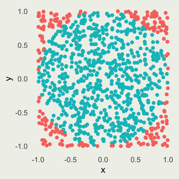
• Imagine that we need to find the values of the slope and intercept such that the yellow line fits “nicely” through the cloud of points

• Suppose you have linear regression model of the form \(y_n \sim \operatorname{normal}(\alpha + \beta x_n, \, \sigma)\) and you want to learn the most likely values of \(\alpha\) and \(\beta\)

• The most likely values for slope (beta) and intercept (alpha) are at the peak of this function, which can be found by using (partial) derivatives

Example: Integral Calculus

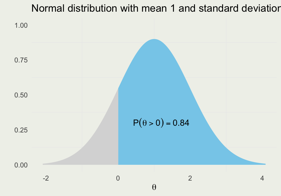
• Suppose we have a probability distribution of some parameter \(\theta\), which represents the differences between the treated and control units

• Further, suppose that \(\theta > 0\) favors the treatment group

• We want to know the probability that treatment is better than control

• This probability can be written as:

\[ \P(\theta > 0) = \int_{0}^{\infty} p_{\theta}\, \text{d}\theta \]

• Assuming \(\theta\) is normally distributed with \(\mu = 1\) and \(\sigma = 1\) we can evaluate the integral as an area under the normal curve from \(0\) to \(\infty\).

Example: Linear Regression

Notice a Linear Algebra notation \(X \beta\), which is matrix-vector multiplication.

data {
  int<lower=0> N;   // number of data items
  int<lower=0> K;   // number of predictors
  matrix[N, K] X;   // predictor matrix
  vector[N] y;      // outcome vector
}
parameters {
  real alpha;           // intercept
  vector[K] beta;       // coefficients for predictors
  real<lower=0> sigma;  // error scale
}
model {
  y ~ normal(X * beta + alpha, sigma);  // likelihood
}

Stan is a probabilistic programming language. You write your data-generating process (model), and Stan performs inference for all the unknowns.

Example: Bionomial Regression

This is the type of model we fit to the O-Rings data.

data {
  int<lower=0> N_rows; // number of rows in data
  int<lower=0> N;      // number of possible "successes" in Binom(N, p)
  vector[N_rows] x;    // temperature for the O-Rings example
  array[N_rows] int<lower=0, upper=N> y; // number of "successes" in y ~ Binom(N, p)
}
parameters {
  real alpha; 
  real beta;  
}
model {
  alpha ~ normal(0, 2.5); // we can encode what we know about plausible values
  beta ~ normal(0, 1);    // of alpha and beta prior to conditioning on the data
  y ~ binomial_logit(N, alpha + beta * x); // likehood (conditioned on x)
}

\[ \begin{eqnarray*} \text{BinomialLogit}(y~|~N,\theta) & = & \text{Binomial}(y~|~N,\text{logit}^{-1}(\theta)) \\[6pt] & = & \binom{N}{y} \left( \text{logit}^{-1}(\theta) \right)^{y} \left( 1 - \text{logit}^{-1}(\theta) \right)^{N - y} \end{eqnarray*} \]

Example: IRT Model

Item-Response Theory models are popular in education research but generalize to other applications.

data {
  int<lower=1> J;                     // number of students
  int<lower=1> K;                     // number of questions
  int<lower=1> N;                     // number of observations
  array[N] int<lower=1, upper=J> jj;  // student for observation n
  array[N] int<lower=1, upper=K> kk;  // question for observation n
  array[N] int<lower=0, upper=1> y;   // correctness for observation n
}
parameters {
  real delta;            // mean student ability
  array[J] real alpha;   // ability of student j - mean ability
  array[K] real beta;    // difficulty of question k
}
model {
  alpha ~ std_normal();         // informative true prior
  beta ~ std_normal();          // informative true prior
  delta ~ normal(0.75, 1);      // informative true prior
  for (n in 1:N) {
    y[n] ~ bernoulli_logit(alpha[jj[n]] - beta[kk[n]] + delta);
  }
}

Analysis Environment

• Instructions for installing R and RStudio
• Install the latest version of R
• Install the latest version of the RStudio Desktop
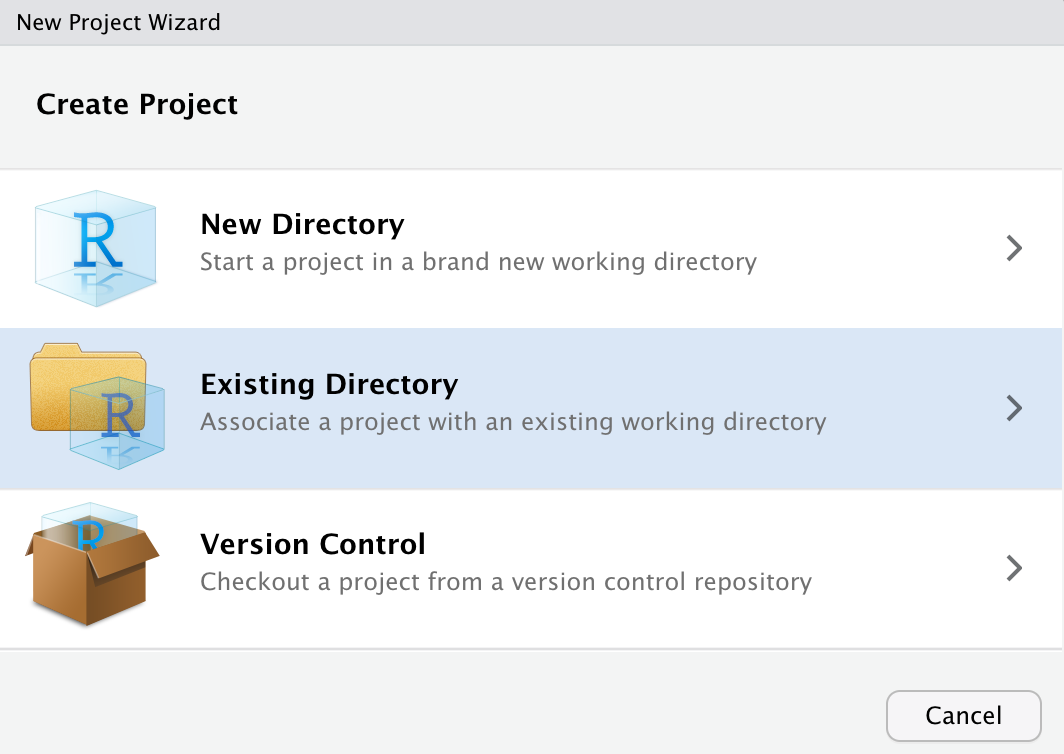
• Create a directory on your hard drive and give it a simple name. Mine is called statsmath
• In RStudio, go to File -> New Project and select: “Existing Directory”
• How many of you have not used RStudio?

What is R

• R is an open-source, interpreted, weakly typed, (somewhat) functional programming language

• R is an implementation of the S language developed at Bell Labs around 1976

• Ross Ihaka and Robert Gentleman started working on R in the early 1990s

• Version 1.0 was released in 2000

• There are ~20,000+ R packages available on CRAN

• R has a large and mostly friendly user community

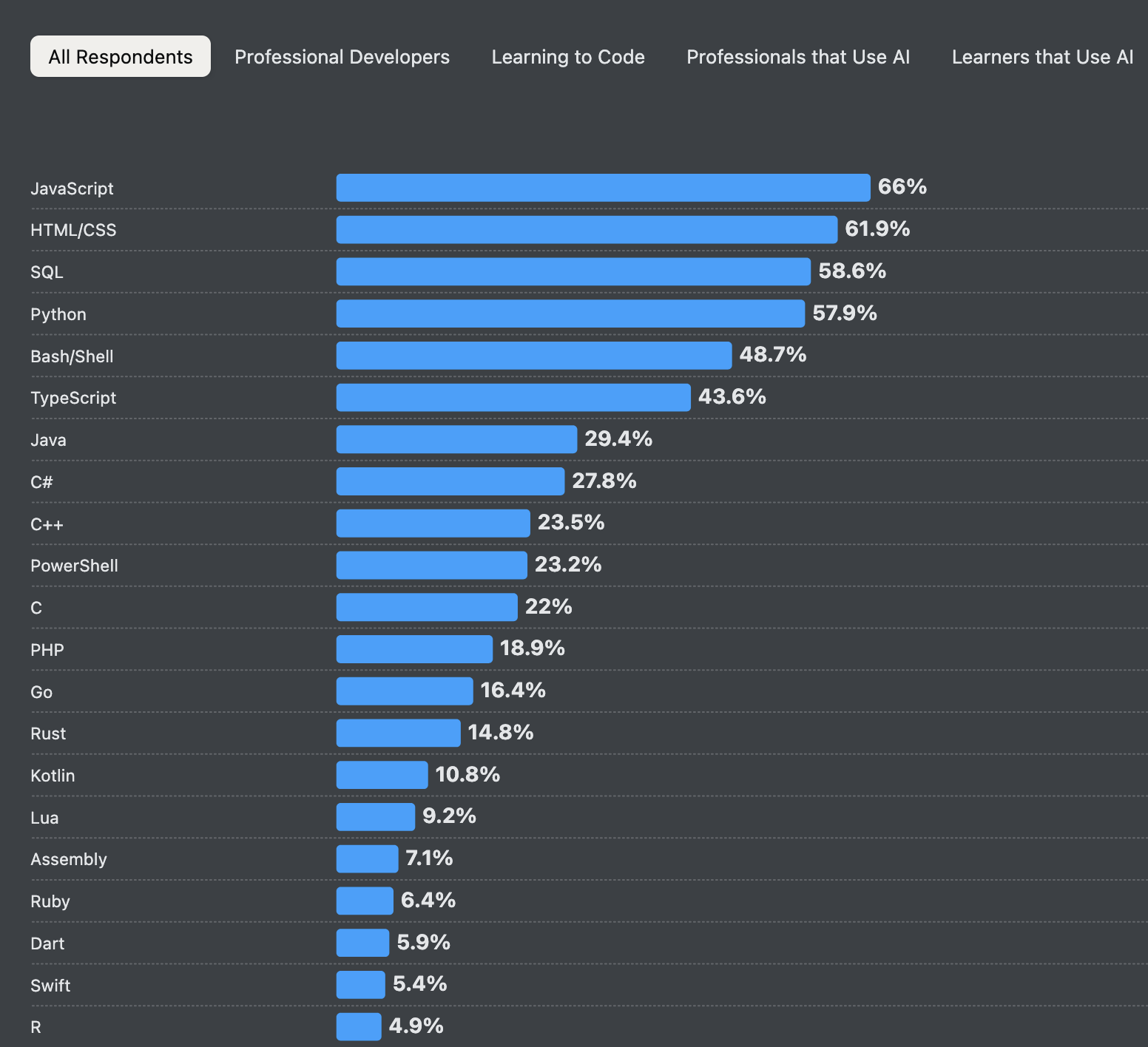Source: StackOverflow Developer Survey

Hands-On: Very Basics

2 + 3

[1] 5

10^3

[1] 1000

10 - 5 / 2

[1] 7.5

(10 - 5) / 2

[1] 2.5

1:10

 [1]  1  2  3  4  5  6  7  8  9 10

1:10 + 1

 [1]  2  3  4  5  6  7  8  9 10 11

sin(pi/2) + cos(pi/2)

[1] 1

1i

[1] 0+1i

round(exp(1i * pi) + 1)

[1] 0+0i

(exp(1i * pi) + 1) |> round()

[1] 0+0i

die <- 1:6
die <- seq(1, 6, by = 1)
die

[1] 1 2 3 4 5 6

length(die) 

[1] 6

str(die)     

 num [1:6] 1 2 3 4 5 6

sum(die)

[1] 21

prod(die)

[1] 720

mean(die)

[1] 3.5

sum(die) / length(die)

[1] 3.5

median(die)

[1] 3.5

sd(die)

[1] 1.870829

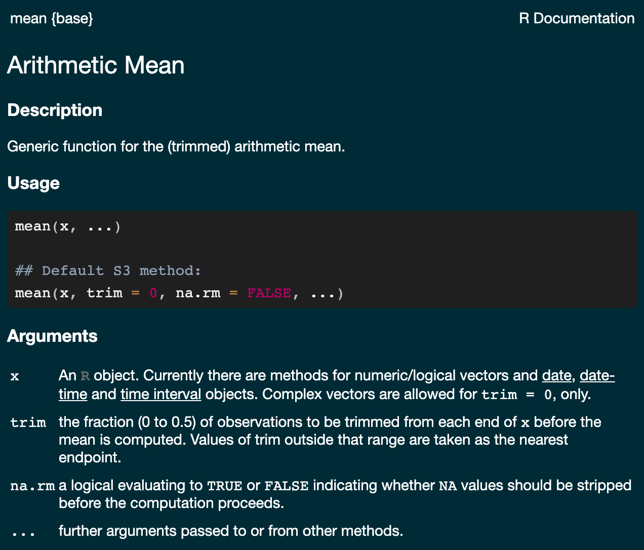
R Documentation

?mean # same as help(mean)

Your Turn

• Create a variable called fib that contains the first 10 Fibonacci numbers
• They are: 0, 1, 1, 2, 3, 5, 8, 13, 21, 34
• Compute the length of this vector in R
• Compute the sum, the product, and the difference (diff()) between successive numbers
• What do you notice about the pattern in the differences?
• Now, create a vector of 100 integers from 1 to 100
• Young Gauss (allegedly) was asked to sum them by hand
• He figured out that the sum has to be \(N (N + 1) / 2\)
• Verify that Gauss was right (just for 100)
• Now compute the sum of the first hundred squares

Hands-On: Lists

• Lists are collections of objects of different types and shapes
• Contrast with a data frame, which we will discuss later, that contains objects of different types but is rectangular

list_x <- list(A = pi, B = c(0, 1), C = 1:10, D = c("one", "two"))
list_x

$A
[1] 3.141593

$B
[1] 0 1

$C
 [1]  1  2  3  4  5  6  7  8  9 10

$D
[1] "one" "two"

str(list_x)

List of 4
 $ A: num 3.14
 $ B: num [1:2] 0 1
 $ C: int [1:10] 1 2 3 4 5 6 7 8 9 10
 $ D: chr [1:2] "one" "two"

list_x$A

[1] 3.141593

list_x[1]

$A
[1] 3.141593

str(list_x[1])

List of 1
 $ A: num 3.14

list_x[[1]] # same as x$A

[1] 3.141593

Data Frames

• Data frames are rectangular structures that are often used in data analysis

• There is a built-in function called data.frame, but we recommend tibble, which is part of the dplyr package

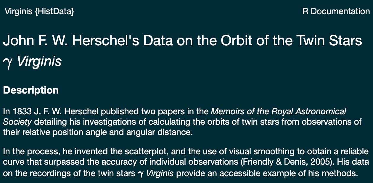
• You can look up the documentation of any R function this way: ?dplyr::tibble. If the package is loaded by using library(dplyr) you can omit dplyr:: prefix

• John F. W. Herschel’s data on the orbit of the Twin Stars \(\gamma\) Virginis

Data Frames

library(HistData)
data("Virginis.interp")
class(Virginis.interp)

[1] "data.frame"

Virginis.interp |> dplyr::as_tibble()

# A tibble: 14 × 4
    year posangle distance velocity
   <int>    <dbl>    <dbl>    <dbl>
 1  1720    160      17.2    -0.32 
 2  1730    157.     16.8    -0.354
 3  1740    153      16.3    -0.376
 4  1750    149.     15.5    -0.416
 5  1760    144.     14.5    -0.478
 6  1770    140.     13.7    -0.533
 7  1780    134.     13.5    -0.547
 8  1790    129.     12.9    -0.597
 9  1800    122.     12.6    -0.632
10  1810    116.     11.2    -0.8  
11  1815    111.     10.4    -0.929
12  1820    106.      9.57   -1.09 
13  1825     98.3     7.09   -1.99 
14  1830     84.3     4.9    -4.16 

Virginis.interp |> dplyr::as_tibble() |> class()

[1] "tbl_df"     "tbl"        "data.frame"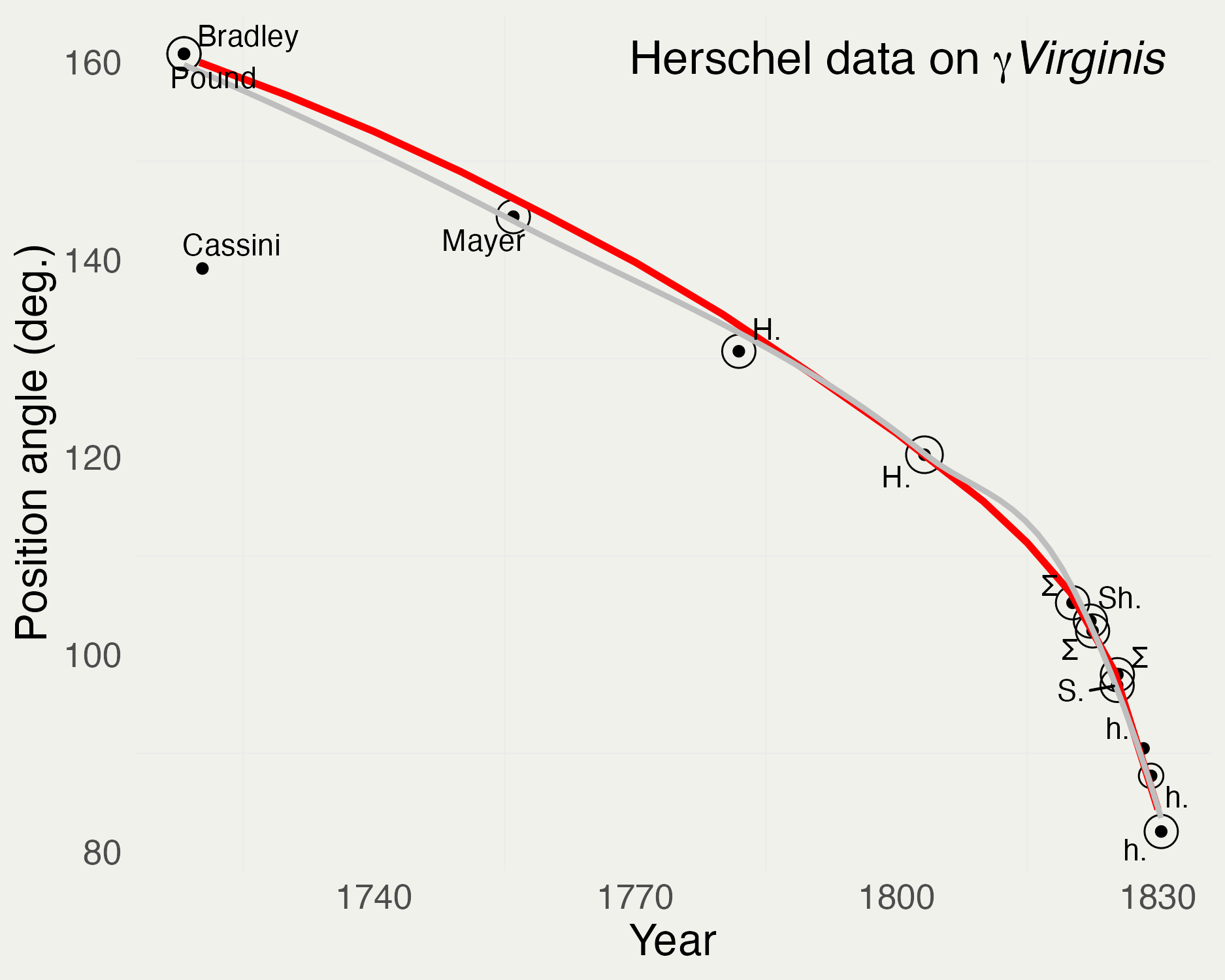

Code for generated the above plot can be found here.

Your Turn

• Save Virginis.interp in a new tibble called virginis using as_tibble() function
• Compute average velocity in virginis
• Hint: you can access columns of tibbles and data frames with an $ like this: dataframe_name$variable_name
• We will do a lot more work with tibbles and data frames in later sessions

Basic Plotting

• John Snow
• Deaths Over Time
• Map of Cholera in London

• R base plotting system is great for making quick graphs with relatively little typing

• In base plot, you add elements to the plot directly, as opposed to describing how the graph is constructed

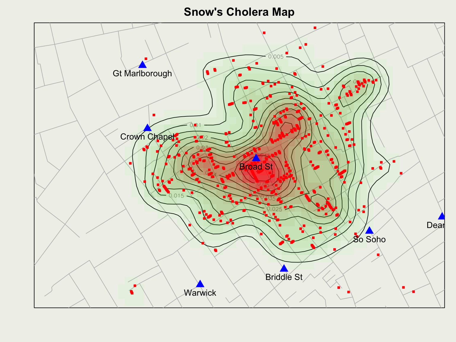
• We will demonstrate with John Snow’s data from the 1854 cholera outbreak

library(HistData)
library(lubridate)

# set up the plotting area so it looks nice
par(mar = c(3, 3, 2, 1), mgp = c(2, .7, 0), 
    tck = -.01, bg = "#f0f1eb")
clr <- ifelse(Snow.dates$date < mdy("09/08/1854"), 
              "red", "darkgreen")
plot(deaths ~ date, data = Snow.dates, 
     type = "h", lwd = 2, col = clr, xlab = "")
points(deaths ~ date, data = Snow.dates, 
       cex = 0.5, pch = 16, col = clr)
text(mdy("09/08/1854"), 40, 
     "Pump handle\nremoved Sept. 8", pos = 4)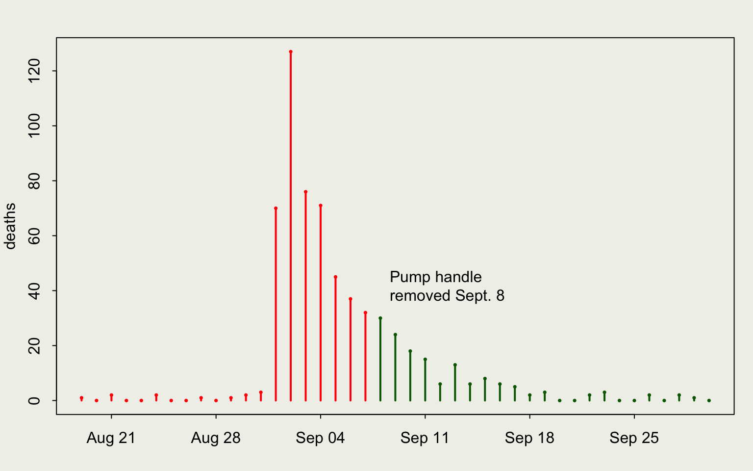

Hands-On: Simulating Coin Flips

We can learn a lot through simulation. We will start with the sample() function.

sample(x, size, replace = FALSE, prob = NULL)

# simulating coin flips
coin <- c("H", "T")

# flip a fair coin 10 times; try it with replace = FALSE
sample(coin, 10, replace = TRUE)

 [1] "H" "T" "T" "H" "T" "T" "H" "H" "H" "T"

# flip a coin that has P(H = 0.6) 10 times
sample(coin, 10, replace = TRUE, prob = c(0.6, 0.4))

 [1] "T" "H" "H" "T" "T" "H" "H" "T" "H" "H"

# it's more convenient to make H = 1 and T = 0
coin <- c(1, 0)
sample(coin, 10, replace = TRUE)

 [1] 1 0 1 1 1 0 0 1 1 1

• Your turn: flip a coin 1000 times and compute the proportion of heads

For Loops

• For Loops
• Solution

• Suppose you want to add the first 100 integers as before but without using the sum() function or the formula
• In math notation: \(\sum_{i = 1}^{100}x_i\), \(\mathbf{x} = (1, 2, 3, \dots, 100)\)

n <- 100
x <- 1:n
s <- 0
for (i in 1:n) {
  s <- s + x[i] 
}
# test
s == sum(x)

[1] TRUE

• Your turn: modify the loop to add only even numbers in 1:100. Look up help(if) statement and modulo operator help(%%); write a test to check your work

s <- 0
for (i in 1:n) {
  if (x[i] %% 2 == 0) {
    s <- s + x[i]
  }
}
cat(s)

2550

# test 
s == sum(seq(2, 100, by = 2))

[1] TRUE

• Congratulations, you are now Turing Complete!

Simulate Coin Flips

• If we flip a coin more and more times, would the estimate of the proportion become better?
• If so, what is the rate of convergence?

set.seed(1) # why do we do this?
n <- 1e4
est_prop <- numeric(n) # allocate a vector of size n
for (i in 1:n) {
  x <- sample(coin, i, replace = TRUE)
  est_prop[i] <- mean(x)
}

• Your turn: write down in plain English what the above code is doing
• At the end of the loop, what does the variable est_prop contain?

Introduction to ggplot

• Our task is to visualize the estimated proportion as a function of the number of coin flips
• This can be done in base plot(), but we will do it with ggplot

library(ggplot2)
library(gridExtra)

x <- seq(0, 100, by = 5)
y <- x^2

quadratic <- tibble(x = x, y = y)
p1 <- ggplot(data = quadratic, 
             mapping = aes(x = x, y = y))
p2 <- p1 + geom_point(size = 0.5)
p3 <- p1 + geom_line(linewidth = 0.2, 
                     color = 'red')
p4 <- p1 + geom_point(size = 0.5) + 
  geom_line(linewidth = 0.2, color = 'red')

grid.arrange(p1, p2, p3, p4, nrow = 2)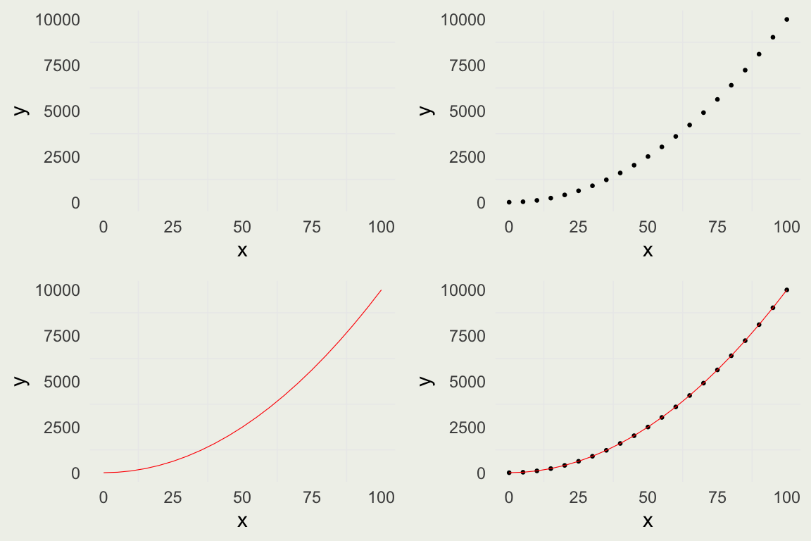

Law of Large Numbers

• Code
• Plot

set.seed(1) 
n <- 1e4
est_prop <- numeric(n) 
for (i in 1:n) {
  x <- sample(coin, i, replace = TRUE)
  est_prop[i] <- mean(x)
}

library(scales)
data <- tibble(num_flips = 1:n, est_prop = est_prop)
p <- ggplot(data = data, mapping = aes(x = num_flips, y = est_prop))
p + geom_line(size = 0.1) + 
  geom_hline(yintercept = 0.5, size = 0.2, color = 'red') +
  scale_x_continuous(trans = 'log10', label = comma) +
  xlab("Number of flips on Log10 scale") +
  ylab("Estimated proportion of Heads") +
  ggtitle("Error decreases with the size of the sample")

We can see some evidence for the Law of Large Numbers.

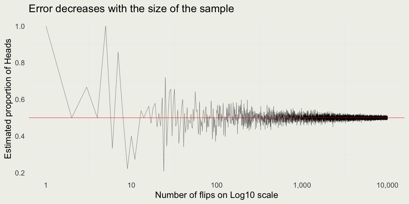
WLLN: \(\lim_{n \to \infty} \mathbb{P}\left( \left| \overline{X}_n - \mu \right| \geq \epsilon \right) = 0\)

Functions

• Structure
• Writing Your Own Function
• Coin Flip Example

• Functions help you break up the code into self-contained, understandable pieces.

• Functions take in arguments and return results. You saw functions like sum() and mean() before. Here, you will learn how to write your own.

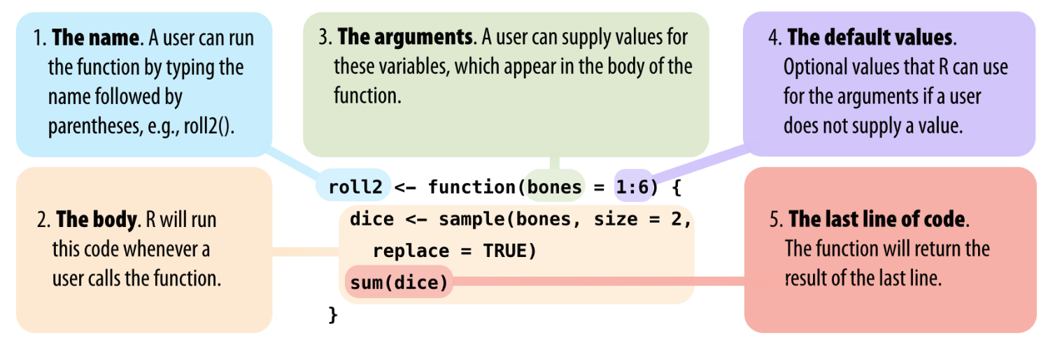
We will write a function that produces one estimate of the proportion given a fixed sample size n.

estimate_proportion <- function(n) {
  coin <- c(1, 0)
  x <- sample(coin, n, replace = TRUE)
  est <- mean(x)
  return(est)
}
estimate_proportion(10)

[1] 0.4

x <- replicate(1e3, estimate_proportion(10))
head(x)

[1] 0.3 0.7 0.5 0.8 0.5 0.6

hist(x, 
     xlab = "", 
     main = "Distribution of Proportions of Heads")

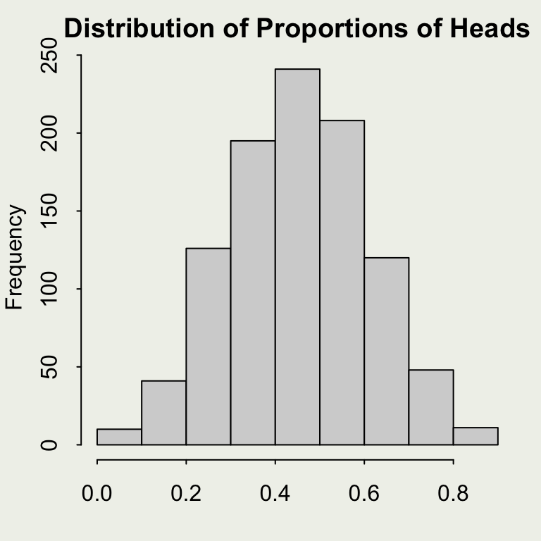
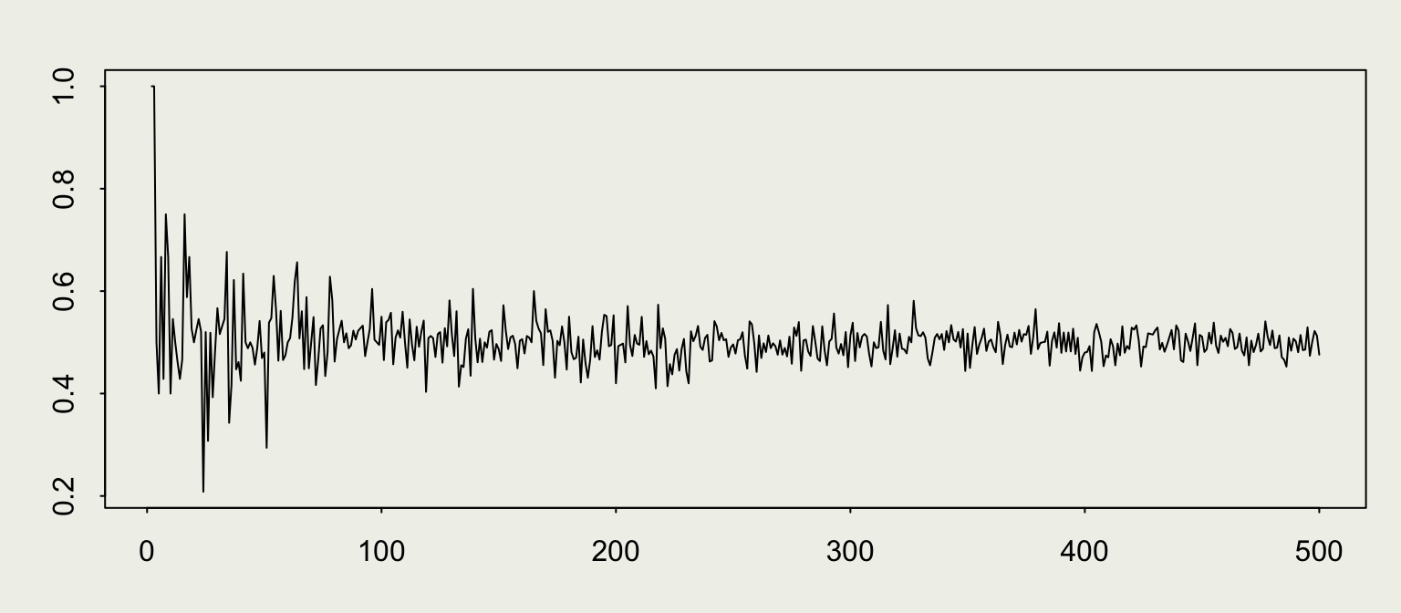
To reproduce our earlier example, generating estimates for increasing sample sizes, use map_dbl() function from purrr package. More on that here.

library(purrr)
par(mar = c(3, 3, 2, 1), mgp = c(2, .7, 0), tck = -.01, bg = "#f0f1eb")
y <- map_dbl(2:500, estimate_proportion)
# above is the same as sapply(2:500, estimate_proportion)
plot(2:500, y, xlab = "", ylab = "", type = 'l')

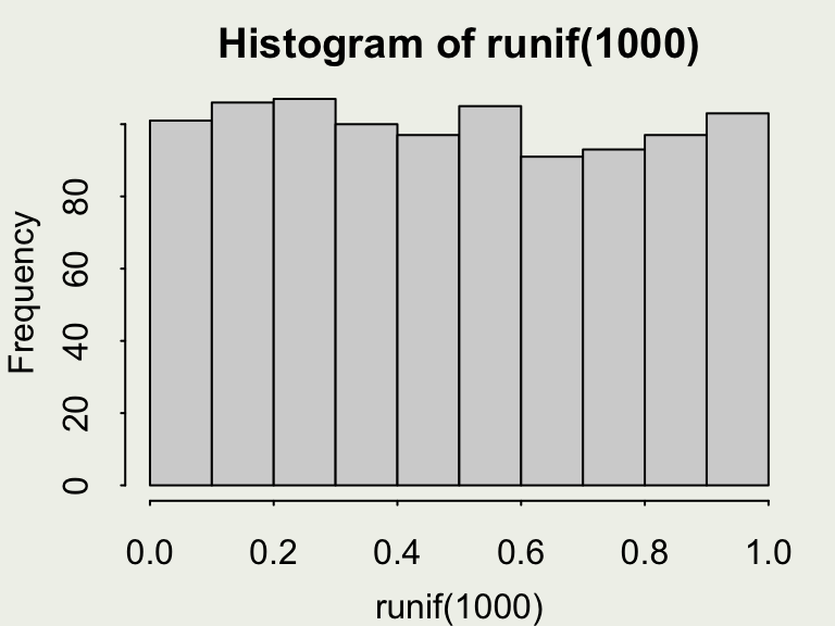
Generating Continuous Uniform Draws

• Here, we will examine a continuous version of the sample() function: runif(n, min = 0, max = 1)
• runif generates realizations of a random variable uniformly distributed between min and max.

• Your turn: what is the approximate value of this line of code: mean(runif(1e3, min = -1, max = 0))? Guess before running it.

Estimating \(\pi\) by Simulation

The idea is that we can approximate the ratio of the area of an inscribed circle, \(A_c\), to the area of the square, \(A_s\), by uniformly “throwing darts” at the square with the side \(2r\) and counting how many darts land inside the circle versus inside the square.

\[ \begin{align} A_{c}& = \pi r^2 \\ A_{s}& = (2r)^2 = 4r^2 \\ \frac{A_{c}}{A_{s}}& = \frac{\pi r^2}{4r^2} = \frac{\pi}{4} \implies \pi = \frac{4A_{c}}{A_{s}} \end{align} \]

Estimating \(\pi\) by Simulation

To estimate \(\pi\), we perform the following simulation:

\[ \begin{align} X& \sim \text{Uniform}(-1, 1) \\ Y& \sim \text{Uniform}(-1, 1) \\ \pi& \approx \frac{4 \sum_{i=1}^{N} \I(x_i^2 + y_i^2 < 1)}{N} \end{align} \]

The numerator is a sum over an indicator function \(\I\), which evaluates to \(1\) if the inequality holds and \(0\) otherwise.

Estimating \(\pi\) by Simulation

• Code and Plot
• Estimate

n <- 1e3
x <- runif(n, -1, 1); y <- runif(n, -1, 1)
inside <- x^2 + y^2 < 1
data <- tibble(x, y, inside)
p <- ggplot(aes(x = x, y = y), data = data)
p + geom_point(aes(color = inside)) + theme(legend.position = "none")

cat("Estimated value of pi =", 4*sum(inside) / n)

Estimated value of pi = 3.112

x	y	inside
-0.8287282	-0.2198830	TRUE
-0.9964402	0.4200821	FALSE
-0.1473951	-0.1864385	TRUE
0.6455366	0.6547743	TRUE
0.7709646	-0.9771841	FALSE

References

Blitzstein, Joseph K., and Jessica Hwang. 2019. Introduction to Probability. Second edition. Crc Press/Taylor & Francis Group.

Boyd, Stephen P., and Lieven Vandenberghe. 2018. Introduction to Applied Linear Algebra: Vectors, Matrices, and Least Squares. Cambridge University Press.

Fowlkes, Edward B., and Bruce Hoadley. 1989. “Risk Analysis of the Space Shuttle: Pre-Challenger Prediction of Failure AU - Dalal, Siddhartha r.” Journal of the American Statistical Association 84 (408): 945–57. https://doi.org/10.1080/01621459.1989.10478858.

Grolemund, Garrett. 2014. Hands-on Programming with r. First edition. O’Reilly. https://rstudio-education.github.io/hopr/.

Herman, Edwin, Gilbert Strang, and OpenStax. 2016. Calculus Volume 1. https://d3bxy9euw4e147.cloudfront.net/oscms-prodcms/media/documents/CalculusVolume1-OP.pdf.

Martz, H. F., and W. J. Zimmer. 1992. “The Risk of Catastrophic Failure of the Solid Rocket Boosters on the Space Shuttle.” The American Statistician 46 (1): 42–47. https://doi.org/10.1080/00031305.1992.10475846.

Petersen, Kaare Brandt, and Michael Syskind Pedersen. 2012. The Matrix Cookbook. https://www.freetechbooks.com/the-matrix-cookbook-t435.html.

Sanderson, Grant. 2018a. Essence of Calculus. (YouTube), November 23. https://www.youtube.com/playlist?list=PLZHQObOWTQDMsr9K-rj53DwVRMYO3t5Yr.

Sanderson, Grant. 2018b. Essence of Linear Algebra. (YouTube), November 23. https://www.youtube.com/playlist?list=PLZHQObOWTQDPD3MizzM2xVFitgF8hE_ab.

Thompson, Silvanus P. 1980. Calculus Made Easy: Being a Very-Simplest Introduction to Those Beautiful Methods of Reckoning Which Are Generally Called by the Terrifying Names of the Differential Calculus and the Integral Calculus. 3d ed. St. Martin’s Press.

Wickham, Hadley, Mine Çetinkaya-Rundel, and Garrett Grolemund. 2023. R for Data Science: Import, Tidy, Transform, Visualize, and Model Data. 2nd edition. O’Reilly Media.