APSTA-GE 2006: Applied Statistics for Social Science Research
Eric.Novik@nyu.edu | Summer 2026 | Session 1
“If you want to be a writer, you must do two things above all others: read a lot and write a lot. There’s no way around these two things that I’m aware of, no shortcut.”
Integral calculus: compute probabilities, expectations, Bayesian statistics
Linear algebra: the language for solving many equations at once
Probability: given a (known) population, how likely is this sample
Statistics: given a sample, what are the attributes of a population
Programming and Statistics in the Age of AI
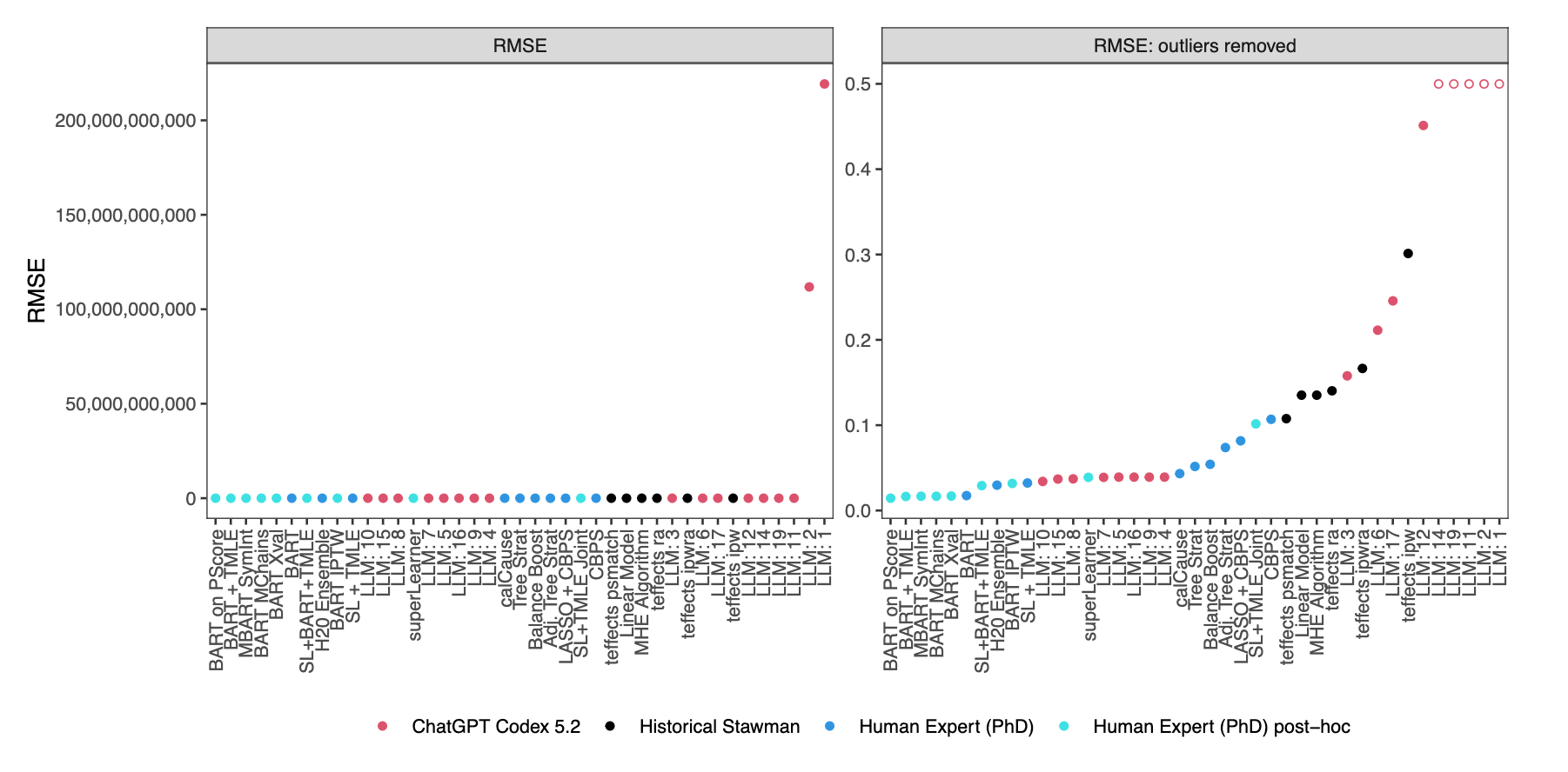
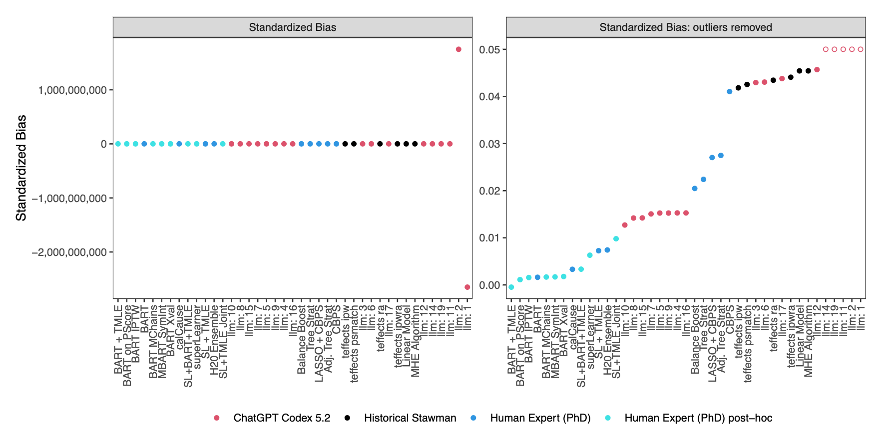
A frontier LLM generated 20 independent solutions to the same statistical programming task. Three did not run, and several that ran produced catastrophic errors.
Each red point is a different ChatGPT Codex 5.2 submission. The worst RMSE exceeded 100 billion outcome standard deviations.
The same prompt produced estimates ranging from competitive to billions of standard deviations from the truth.
The danger is not that every LLM answer is wrong; it is that a plausible-looking answer may be catastrophically wrong. Statistical and programming knowledge lets you verify the output instead of merely trusting it.
Differentiation comes up when you want to find the most likely values of parameters (unknowns) in optimization-based (sometimes called frequentist) inference
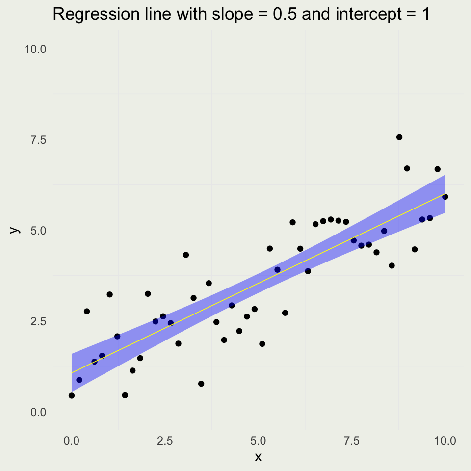
Imagine that we need to find the values of the slope and intercept such that the yellow line fits “nicely” through the cloud of points
Suppose you have linear regression model of the form \(y_n \sim \operatorname{normal}(\alpha + \beta x_n, \, \sigma)\) and you want to learn the most likely values of \(\alpha\) and \(\beta\)
The most likely values for slope (beta) and intercept (alpha) are at the peak of this function, which can be found by using (partial) derivatives
Example: Integral Calculus
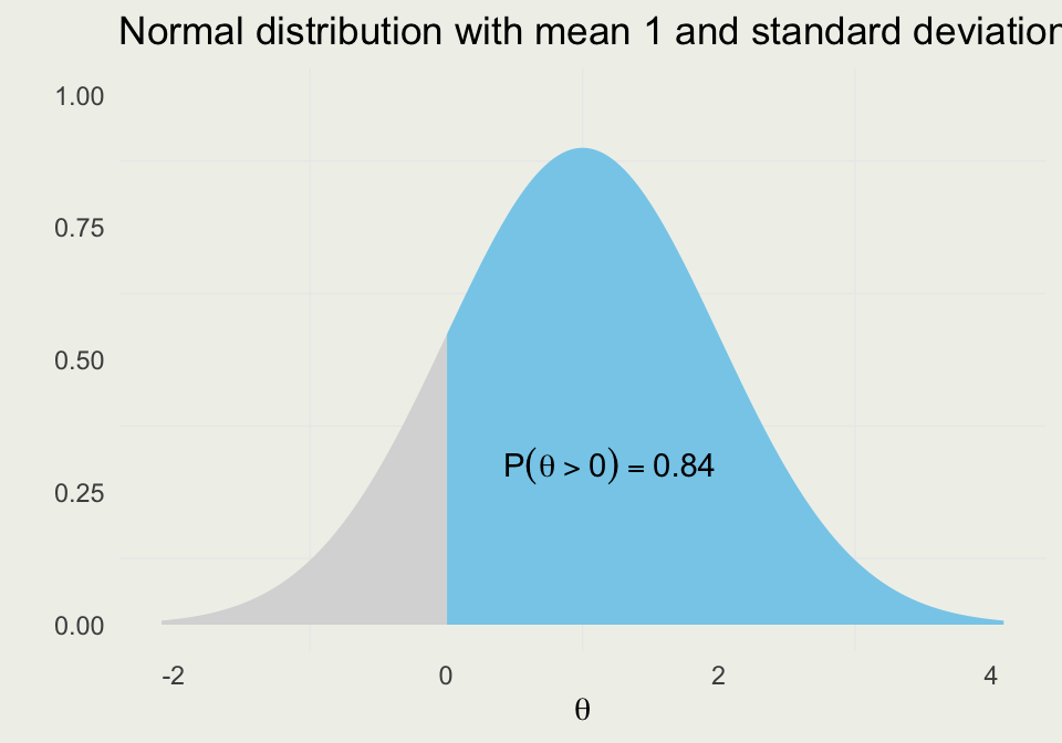
Suppose we have a probability distribution of some parameter \(\theta\), which represents the differences between the treated and control units
Further, suppose that \(\theta > 0\) favors the treatment group
We want to know the probability that treatment is better than control
Assuming \(\theta\) is normally distributed with \(\mu = 1\) and \(\sigma = 1\) we can evaluate the integral as an area under the normal curve from \(0\) to \(\infty\).
Probabilistic Programming
NumPyro
A probabilistic program specifies a forward generative process using random variables and data.
Unknown parameters \(\theta\) (RVs) are represented explicitly; observed data \(x\) and measurements \(y\) condition the model.
An inference engine uses the model to solve the inverse problem (perform inference) without requiring a separate hand-derived solution for every model.
Model specification is separated from algorithms such as numerical optimization (MLE), Hamiltonian Monte Carlo, and variational inference.
R, Python, Julia are not probabilistic programming languages.
Example: Linear Regression
Notice a Linear Algebra notation \(X \beta\), which is matrix-vector multiplication.
Stan
data {int<lower=0> N; // number of data itemsint<lower=0> K; // number of predictorsmatrix[N, K] X; // predictor matrixvector[N] y; // outcome vector}parameters {real alpha; // interceptvector[K] beta; // coefficients for predictorsreal<lower=0> sigma; // error scale}model {// parameters with Normal(0, 1) priors alpha ~ normal(0, 1); beta ~ normal(0, 1);// sigma with Exp(1) prior sigma ~ exponential(1);// likelihood: y ~ normal(X * beta + alpha, sigma) y ~ normal(X * beta + alpha, sigma);}
NumPyro
import numpyroimport numpyro.distributions as distdef model(X, y=None): N, K = X.shape# parameters with Normal(0, 1) priors alpha = numpyro.sample("alpha", dist.Normal(0.0, 1.0)) beta = numpyro.sample("beta", dist.Normal(0.0, 1.0).expand([K]))# sigma with Exp(1) prior sigma = numpyro.sample("sigma", dist.Exponential(1.0))# likelihood: y ~ normal(X * beta + alpha, sigma) mu = X @ beta + alpha numpyro.sample("y", dist.Normal(mu, sigma), obs=y)
Example: Binomial Regression
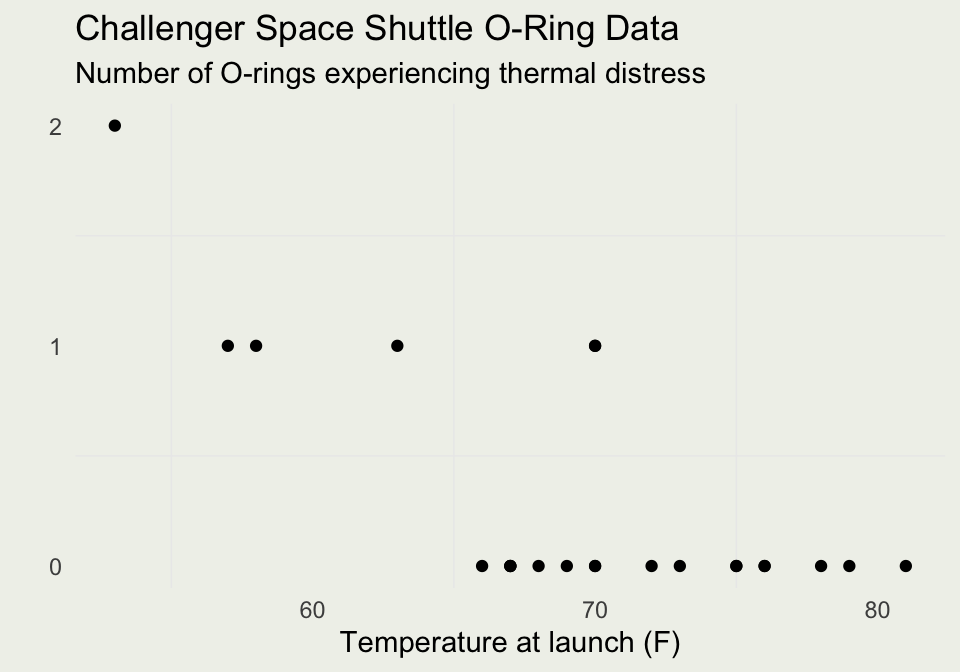
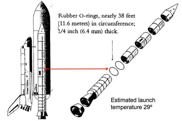
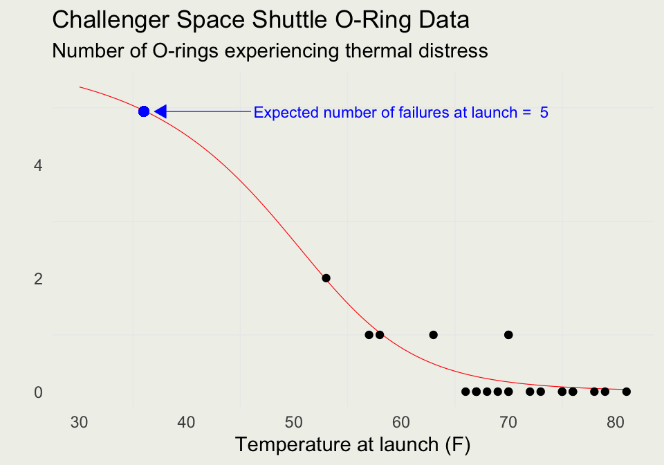
This is the type of model we fit to the O-Rings data.
data {int<lower=0> N_rows; // number of rows in dataint<lower=0> N; // number of possible "successes" in Binom(N, p)vector[N_rows] x; // temperature for the O-Rings examplearray[N_rows] int<lower=0, upper=N> y; // number of "successes" in y ~ Binom(N, p)}parameters {real alpha;real beta;}model { alpha ~ normal(0, 2.5); // we can encode what we know about plausible values beta ~ normal(0, 1); // of alpha and beta prior to conditioning on the data y ~ binomial_logit(N, alpha + beta * x); // likehood (conditioned on x)}
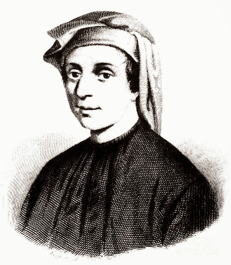
A man put one pair of rabbits in a certain place entirely surrounded by a wall. How many pairs of rabbits can be produced from that pair in a year, if the nature of these rabbits is such that every month each pair bears a new pair which from the second month on becomes productive?
Your Turn
Create a variable called fib that contains the first 10 Fibonacci numbers
They are: 0, 1, 1, 2, 3, 5, 8, 13, 21, 34
Compute the length of this vector in R
Compute the sum, the product, and the difference (diff()) between successive numbers
What do you notice about the pattern in the differences?
Now, create a vector of 100 integers from 1 to 100
Young Gauss (allegedly) was asked to sum them by hand
He figured out that the sum has to be \(N (N + 1) / 2\)
Verify that Gauss was right (just for 100)
Now compute the sum of the first hundred squares
Hands-On: Lists
Lists are collections of objects of different types and shapes
Contrast with a data frame, which we will discuss later, that contains objects of different types but is rectangular
list_x <-list(A = pi, B =c(0, 1), C =1:10, D =c("one", "two"))list_x
List of 4
 $ A: num 3.14
 $ B: num [1:2] 0 1
 $ C: int [1:10] 1 2 3 4 5 6 7 8 9 10
 $ D: chr [1:2] "one" "two"
list_x$A
[1] 3.141593
list_x[1]
$A
[1] 3.141593
str(list_x[1])
List of 1
 $ A: num 3.14
list_x[[1]] # same as x$A
[1] 3.141593
Data Frames
Data frames are rectangular structures that are often used in data analysis
There is a built-in function called data.frame, but we recommend tibble, which is part of the dplyr package
You can look up the documentation of any R function this way: ?dplyr::tibble. If the package is loaded by using library(dplyr) you can omit dplyr:: prefix
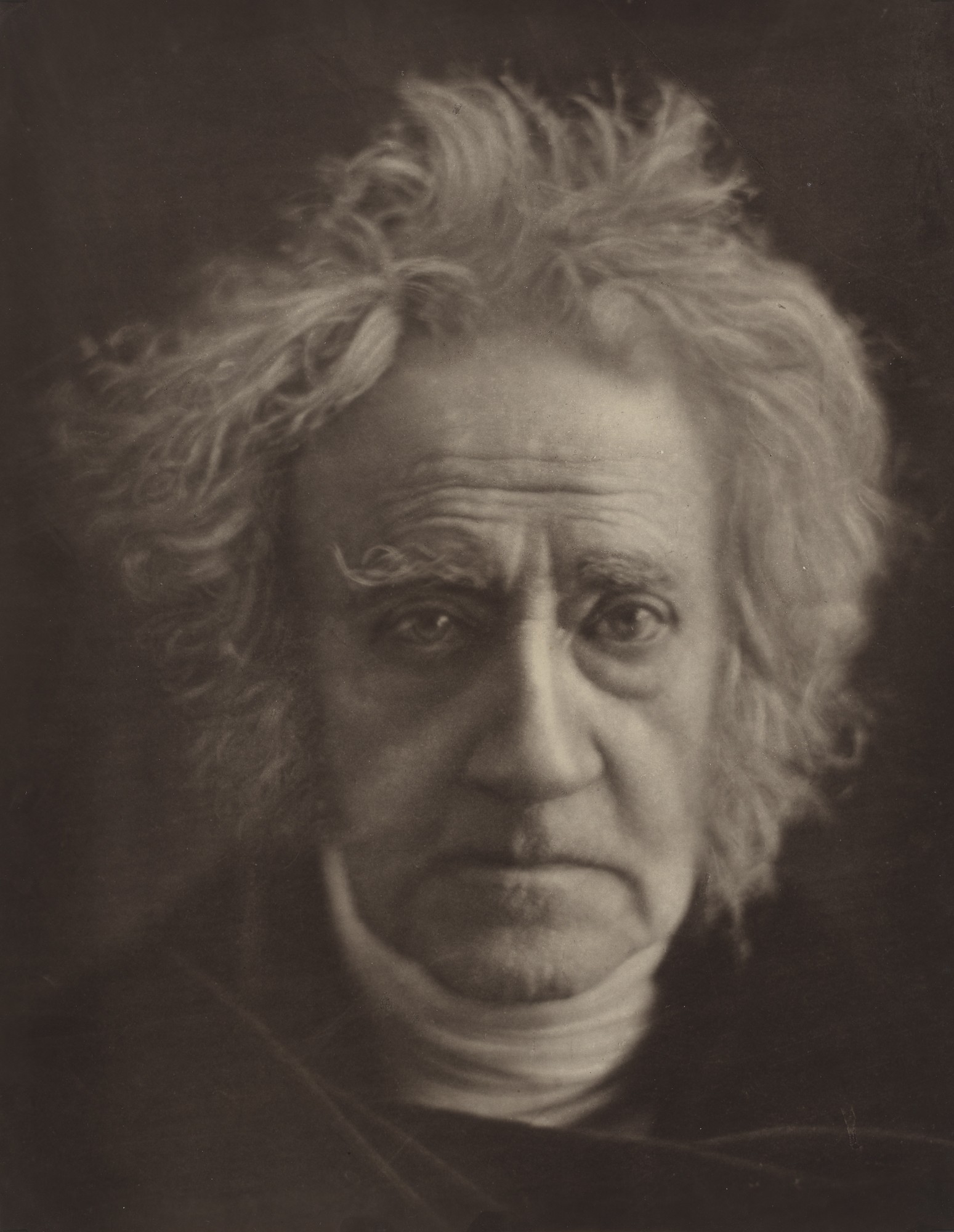
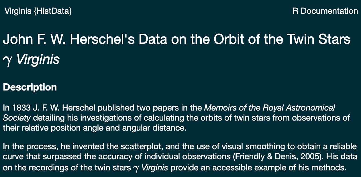
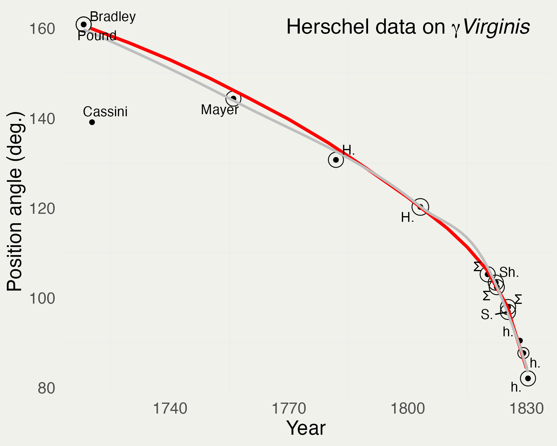
John F. W. Herschel’s data on the orbit of the Twin Stars \(\gamma\) Virginis
If we flip a coin more and more times, would the estimate of the proportion become better?
If so, what is the rate of convergence?
set.seed(1) # why do we do this?n <-1e4est_prop <-numeric(n) # allocate a vector of size nfor (i in1:n) { x <-sample(coin, i, replace =TRUE) est_prop[i] <-mean(x)}
Your turn: write down in plain English what the above code is doing
At the end of the loop, what does the variable est_prop contain?
Introduction to ggplot
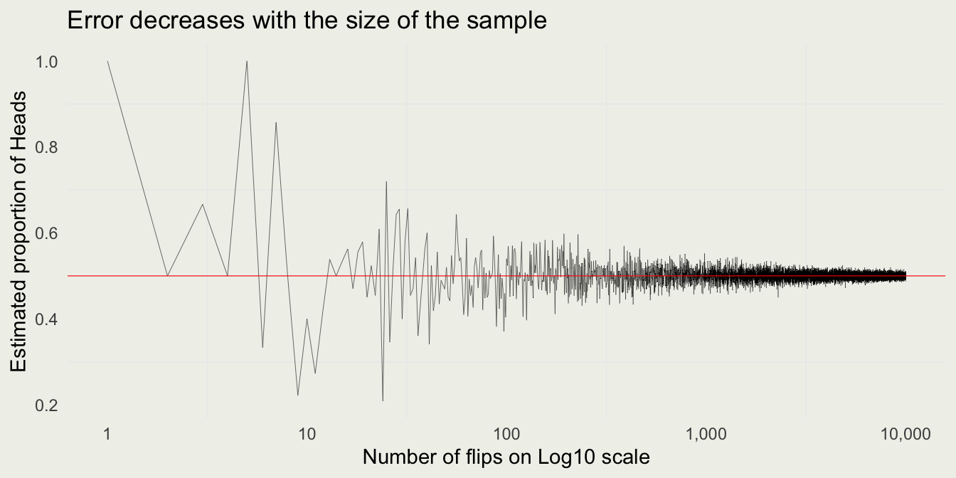
Our task is to visualize the estimated proportion as a function of the number of coin flips
This can be done in base plot(), but we will do it with ggplot
set.seed(1)n <-1e4est_prop <-numeric(n)for (i in1:n) { x <-sample(coin, i, replace =TRUE) est_prop[i] <-mean(x)}library(scales)data <-tibble(num_flips =1:n, est_prop = est_prop)p <-ggplot(data = data, mapping =aes(x = num_flips, y = est_prop))p +geom_line(size =0.1) +geom_hline(yintercept =0.5, size =0.2, color ='red') +scale_x_continuous(trans ='log10', label = comma) +xlab("Number of flips on Log10 scale") +ylab("Estimated proportion of Heads") +ggtitle("Error decreases with the size of the sample")
We can see some evidence for the Law of Large Numbers.
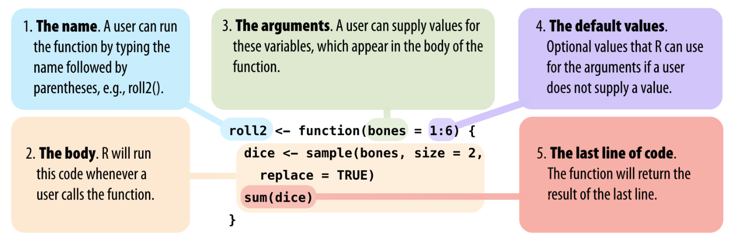
Functions help you break up the code into self-contained, understandable pieces.
Functions take in arguments and return results. You saw functions like sum() and mean() before. Here, you will learn how to write your own.
We will write a function that produces one estimate of the proportion given a fixed sample size n.
estimate_proportion <-function(n) { coin <-c(1, 0) x <-sample(coin, n, replace =TRUE) est <-mean(x)return(est)}estimate_proportion(10)
[1] 0.4
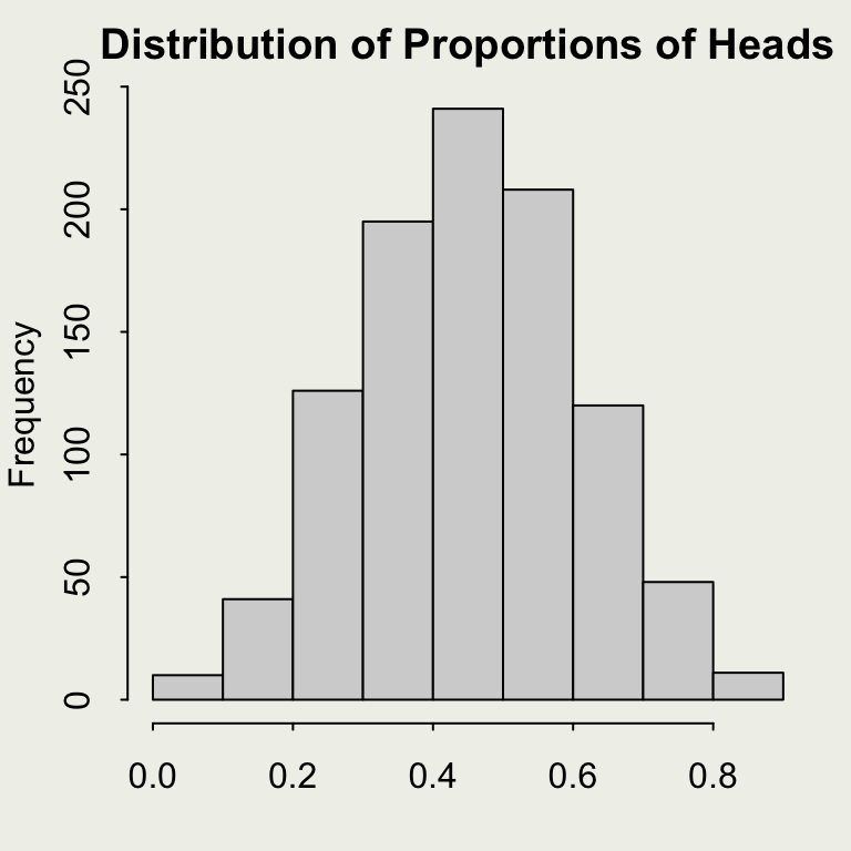
x <-replicate(1e3, estimate_proportion(10))head(x)
[1] 0.3 0.7 0.5 0.8 0.5 0.6
hist(x,xlab ="",main ="Distribution of Proportions of Heads")
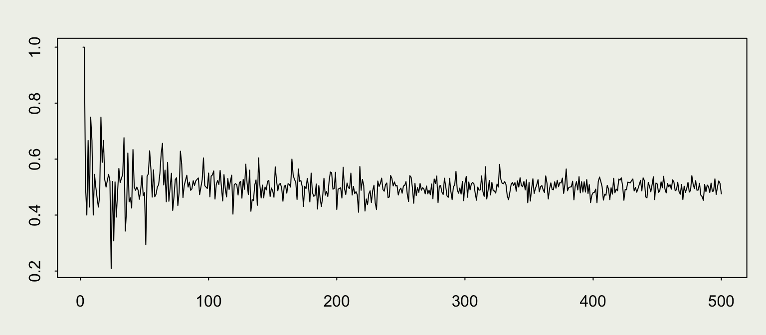
To reproduce our earlier example, generating estimates for increasing sample sizes, use map_dbl() function from purrr package. More on that here.
library(purrr)par(mar =c(3, 3, 2, 1), mgp =c(2, .7, 0), tck =-.01, bg ="#f0f1eb")y <-map_dbl(2:500, estimate_proportion)# above is the same as sapply(2:500, estimate_proportion)plot(2:500, y, xlab ="", ylab ="", type ='l')
Generating Continuous Uniform Draws
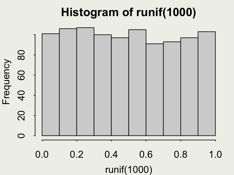
Here, we will examine a continuous version of the sample() function: runif(n, min = 0, max = 1)
runif generates realizations of a random variable uniformly distributed between min and max.
Your turn: what is the approximate value of this line of code: mean(runif(1e3, min = -1, max = 0))? Guess before running it.
Estimating \(\pi\) by Simulation
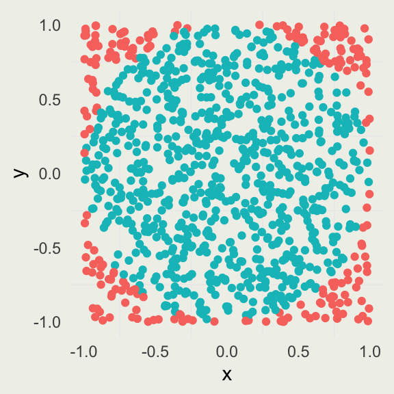
The idea is that we can approximate the ratio of the area of an inscribed circle, \(A_c\), to the area of the square, \(A_s\), by uniformly “throwing darts” at the square with the side \(2r\) and counting how many darts land inside the circle versus inside the square.
Fowlkes, Edward B., and Bruce Hoadley. 1989. “Risk Analysis of the Space Shuttle: Pre-Challenger Prediction of Failure AU - Dalal, Siddhartha r.”Journal of the American Statistical Association 84 (408): 945–57. https://doi.org/10.1080/01621459.1989.10478858.
Martz, H. F., and W. J. Zimmer. 1992. “The Risk of Catastrophic Failure of the Solid Rocket Boosters on the Space Shuttle.”The American Statistician 46 (1): 42–47. https://doi.org/10.1080/00031305.1992.10475846.










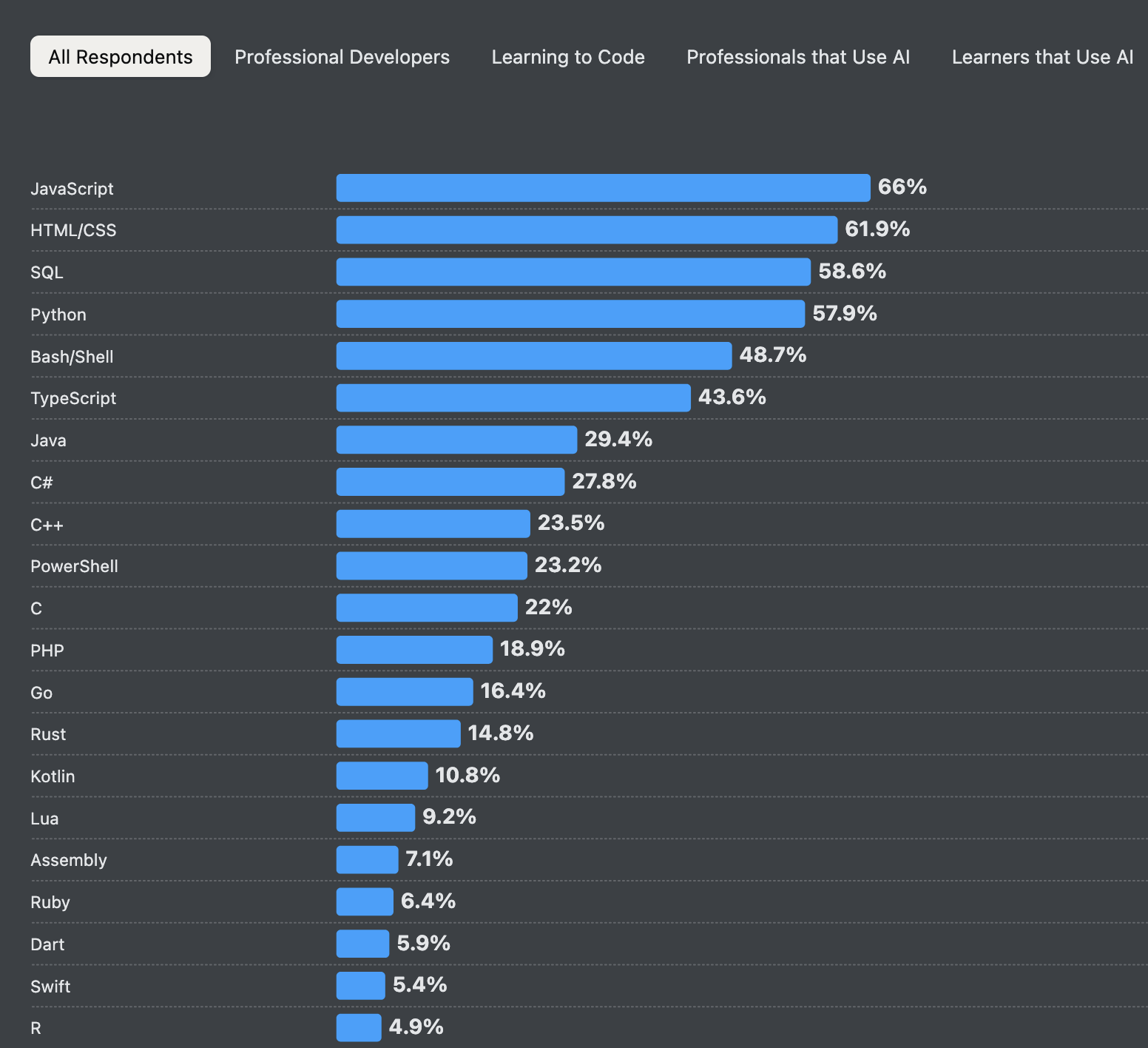 Source: StackOverflow Developer Survey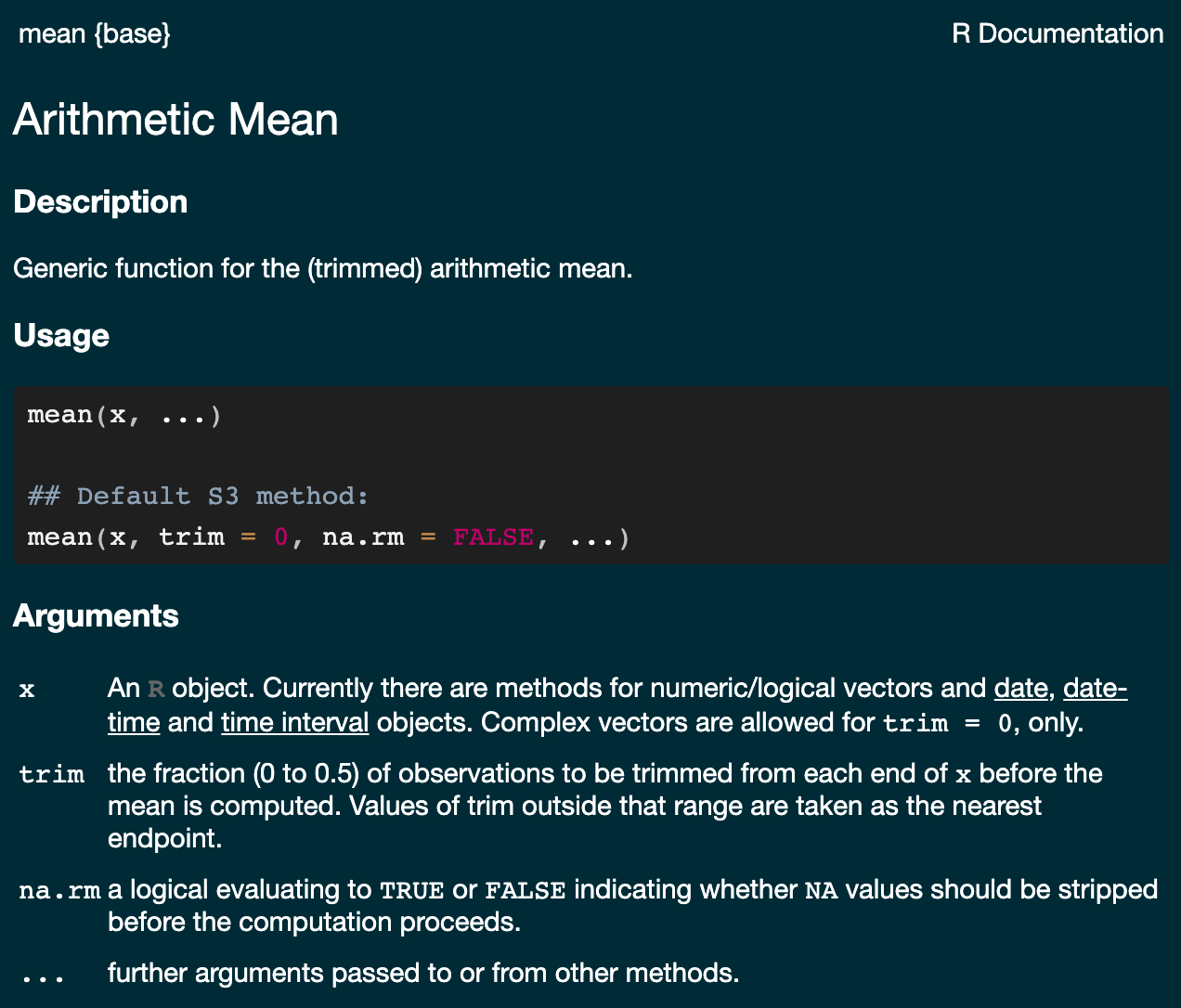
 Code for generated the above plot can be found here.
.jpg)


