APSTA-GE 2006: Applied Statistics for Social Science Research
\[ \DeclareMathOperator{\E}{\mathbb{E}} \DeclareMathOperator{\P}{\mathbb{P}} \DeclareMathOperator{\V}{\mathbb{V}} \DeclareMathOperator{\L}{\mathscr{L}} \DeclareMathOperator{\I}{\text{I}} \]
“If you want to be a writer, you must do two things above all others: read a lot and write a lot. There’s no way around these two things that I’m aware of, no shortcut.”
— Stephen King, On Writing: A Memoir of the Craft
2 × 5 days
30 min
questions
90 min
lecture
60 min
code
Icons: Bootstrap Icons, MIT License.

Big picture
Environment
R project
R console
Syntax
Data
Graphics
Monte Carlo
Icons: Bootstrap Icons, MIT License.


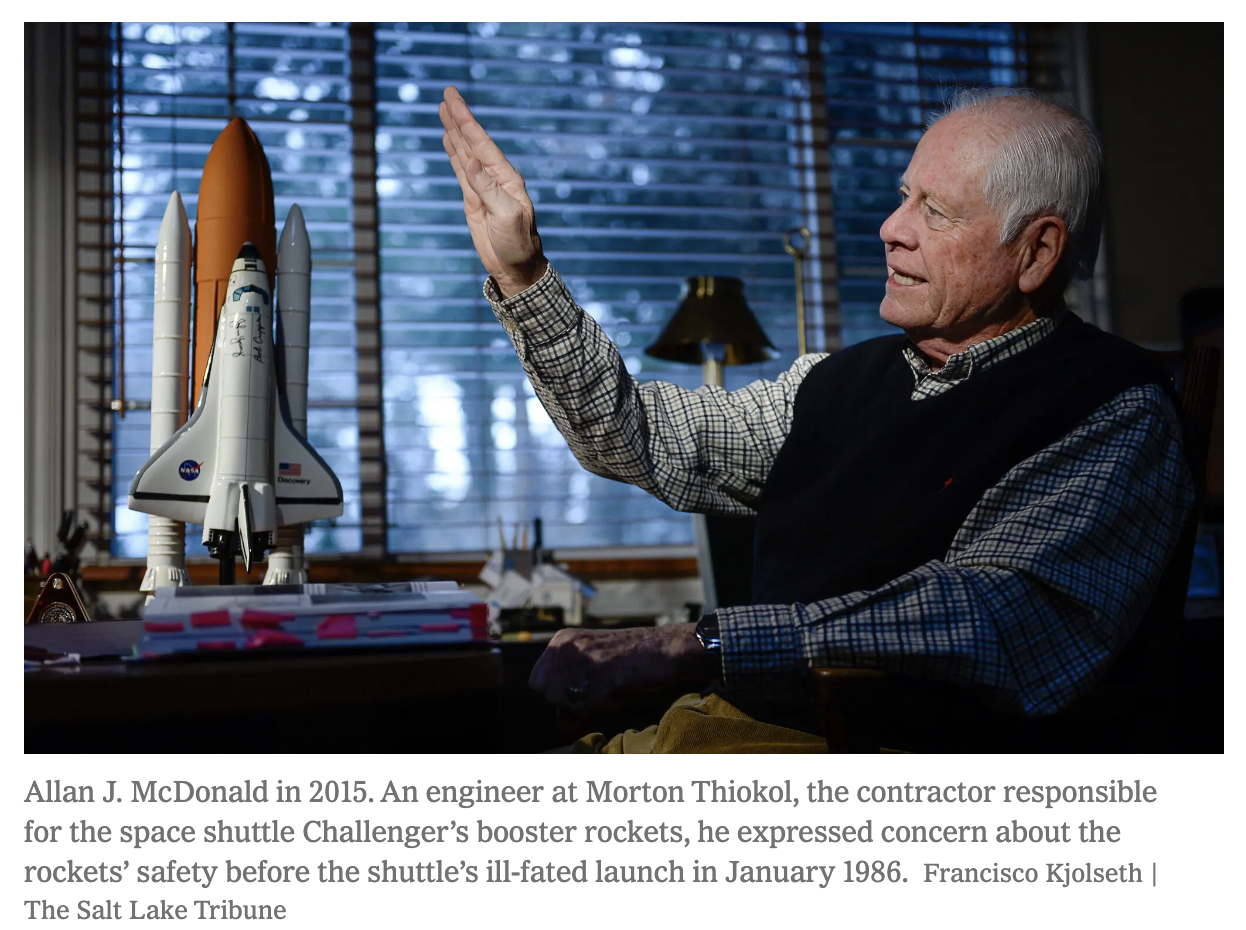
On January 28, 1986, shortly after launch, Shuttle Challenger exploded, killing all seven crew members.
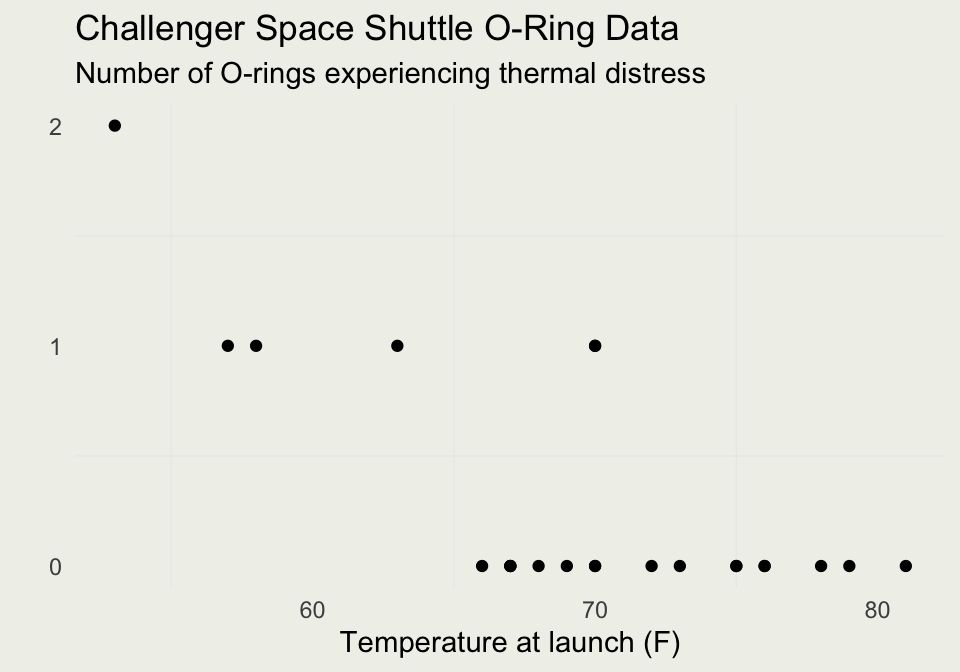
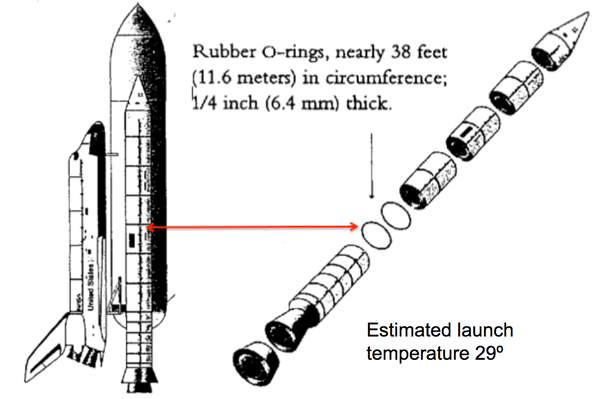
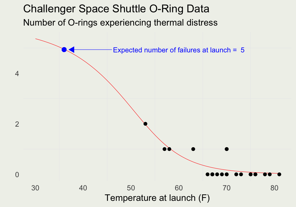
Probability of 1 or more rings being damaged at launch is about 0.99
Probability of all 6 rings being damaged at launch is about 0.46
Data source: UCI Machine Learning Repository


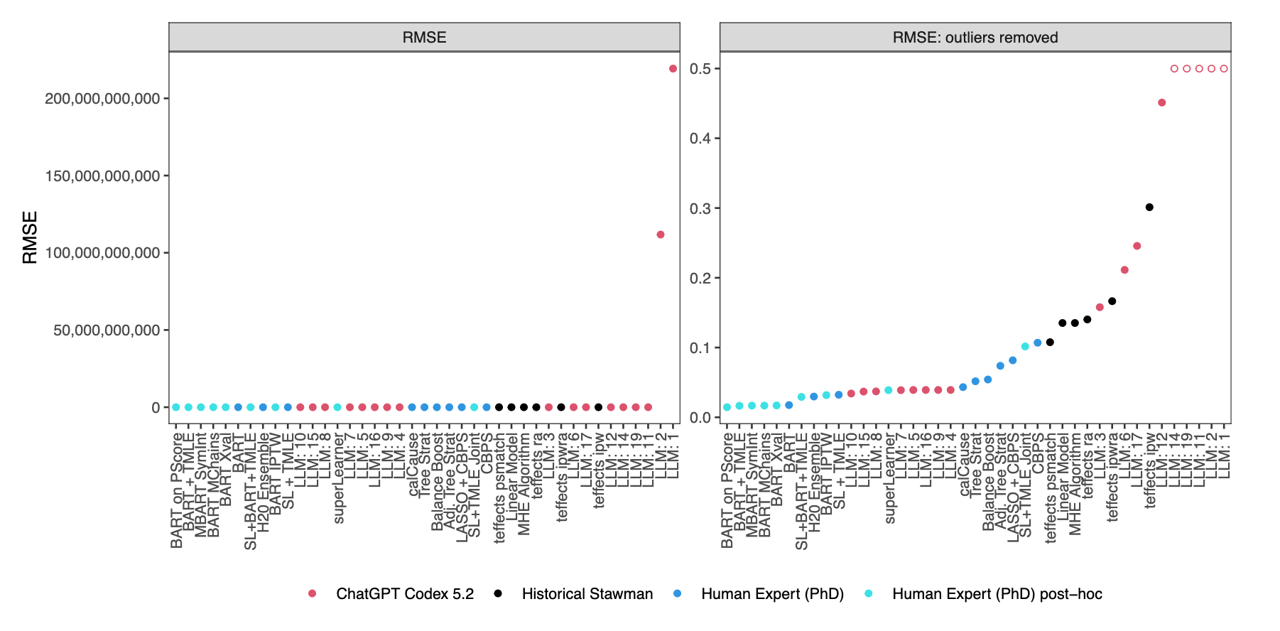
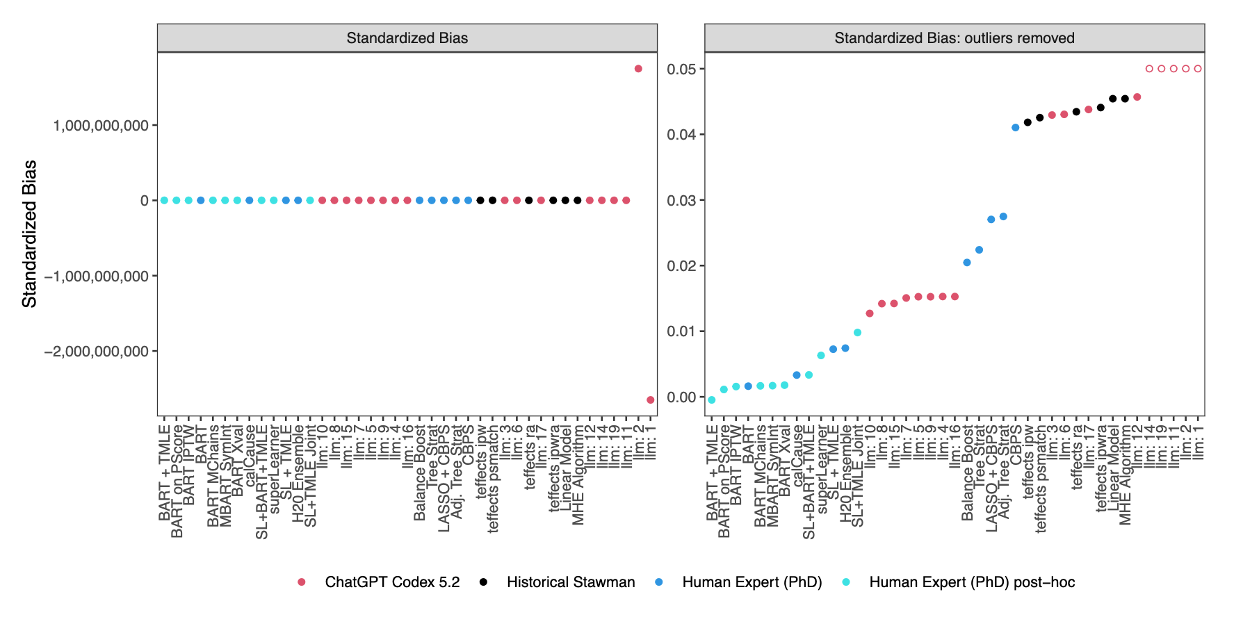
Plot and findings: Perrett, Elliott, Hill, and Scott (2026), Flaws in the LLM Automation Narrative.
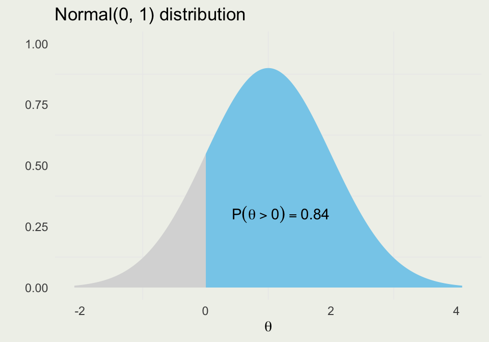
\[ \P(\theta > 0) = \int_{0}^{\infty} p_{\theta}\, \text{d}\theta \]
Notice a Linear Algebra notation \(X \beta\), which is matrix-vector multiplication.
data {
int<lower=0> N; // number of data items
int<lower=0> K; // number of predictors
matrix[N, K] X; // predictor matrix
vector[N] y; // outcome vector
}
parameters {
real alpha; // intercept
vector[K] beta; // coefficients for predictors
real<lower=0> sigma; // error scale
}
model {
// parameters with Normal(0, 1) priors
alpha ~ normal(0, 1);
beta ~ normal(0, 1);
// sigma with Exp(1) prior
sigma ~ exponential(1);
// likelihood
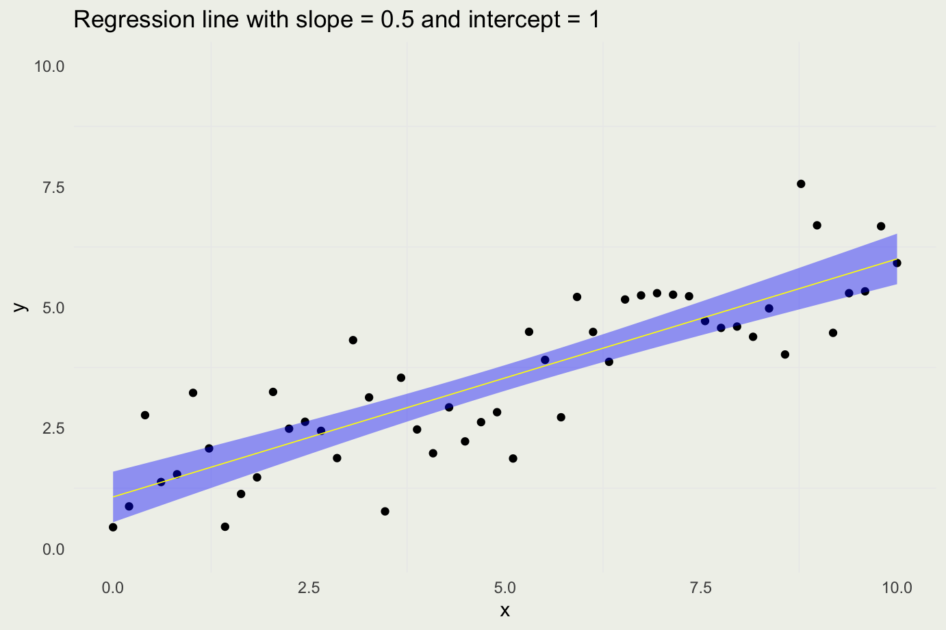
y ~ normal(X * beta + alpha, sigma);
}import numpyro
import numpyro.distributions as dist
def model(X, y=None):
N, K = X.shape
# parameters with Normal(0, 1) priors
alpha = numpyro.sample("alpha", dist.Normal(0.0, 1.0))
beta = numpyro.sample("beta", dist.Normal(0.0, 1.0).expand([K]))
# sigma with Exp(1) prior
sigma = numpyro.sample("sigma", dist.Exponential(1.0))
# likelihood
mu = X @ beta + alpha
numpyro.sample("y", dist.Normal(mu, sigma), obs=y)This is the type of model we fit to the O-Rings data.
data {
int<lower=0> N_rows; // number of rows in data
int<lower=0> N; // number of possible "successes" in Binom(N, p)
vector[N_rows] x; // temperature for the O-Rings example
array[N_rows] int<lower=0, upper=N> y; // number of "successes" in y ~ Binom(N, p)
}
parameters {
real alpha;
real beta;
}
model {
alpha ~ normal(0, 2.5); // we can encode what we know about plausible values
beta ~ normal(0, 1); // of alpha and beta prior to conditioning on the data
y ~ binomial_logit(N, alpha + beta * x); // likehood (conditioned on x)
}\[ \begin{eqnarray*} \text{BinomialLogit}(y~|~N,\theta) & = & \text{Binomial}(y~|~N,\text{logit}^{-1}(\theta)) \\[6pt] & = & \binom{N}{y} \left( \text{logit}^{-1}(\theta) \right)^{y} \left( 1 - \text{logit}^{-1}(\theta) \right)^{N - y} \end{eqnarray*} \]
data {
int<lower=1> J; // number of students
int<lower=1> K; // number of questions
int<lower=1> N; // number of observations
array[N] int<lower=1, upper=J> jj; // student for observation n
array[N] int<lower=1, upper=K> kk; // question for observation n
array[N] int<lower=0, upper=1> y; // correctness for observation n
}
parameters {
real delta; // mean student ability
array[J] real alpha; // ability of student j - mean ability
array[K] real beta; // difficulty of question k
}
model {
alpha ~ std_normal(); // informative true prior
beta ~ std_normal(); // informative true prior
delta ~ normal(0.75, 1); // informative true prior
for (n in 1:N) {
y[n] ~ bernoulli_logit(alpha[jj[n]] - beta[kk[n]] + delta);
}
}\[ \begin{eqnarray*} \text{BernoulliLogit}(y~|~\theta) & = & \text{Bernoulli}(y~|~\text{logit}^{-1}(\theta)) \\[6pt] & = & \left(\text{logit}^{-1}(\theta)\right)^y \left(1-\text{logit}^{-1}(\theta)\right)^{1-y} \end{eqnarray*} \]
1PL item-response model. Source: Stan Manual
R is an open-source, interpreted, weakly typed, (somewhat) functional programming language
R is an implementation of the S language developed at Bell Labs around 1976
Ross Ihaka and Robert Gentleman started working on R in the early 1990s
Version 1.0 was released in 2000
There are ~20,000+ R packages available on CRAN
R has a large and mostly friendly user community
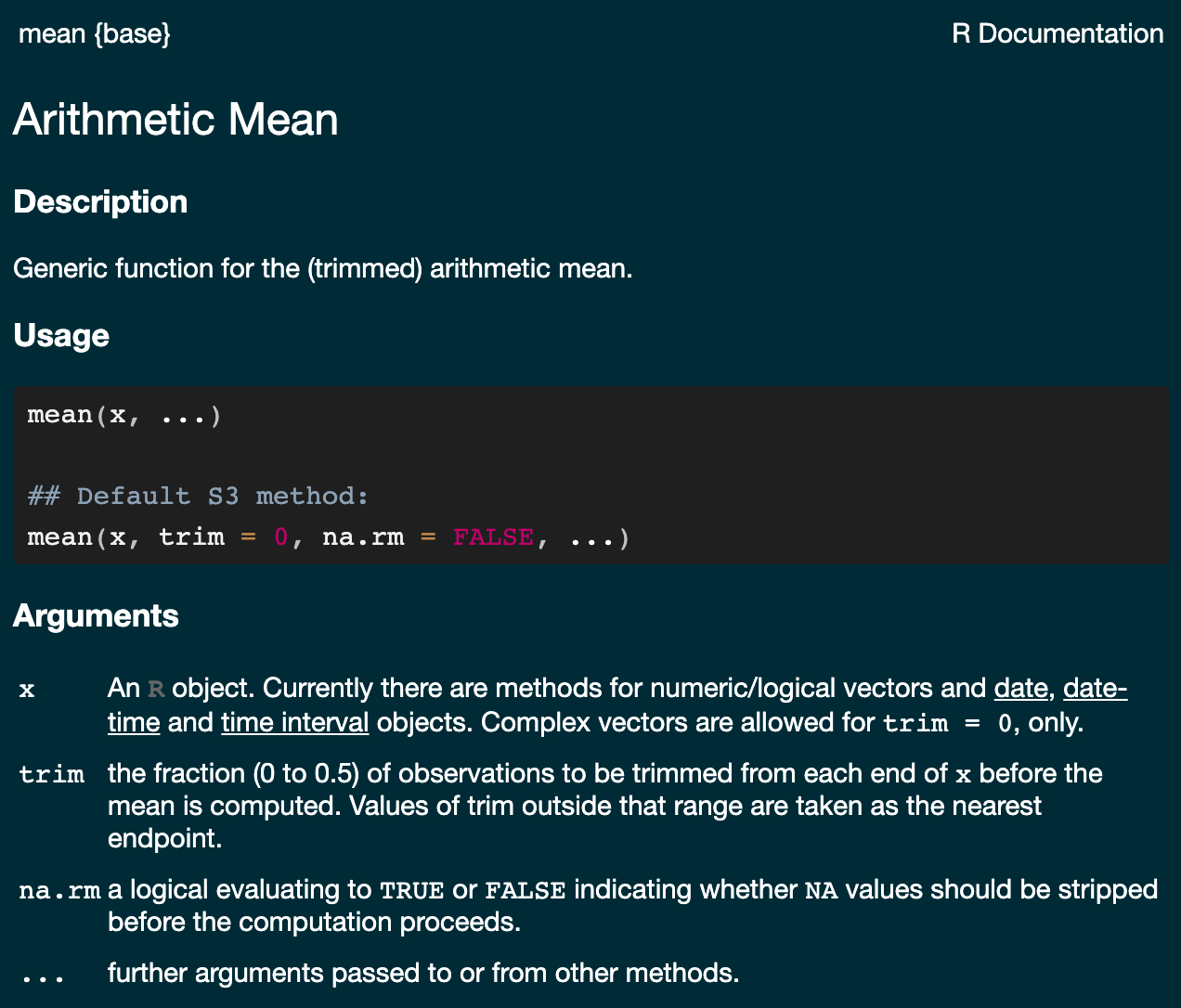
[1] 3.5
[1] 3.5
[1] 3.5
[1] 1.870829
[1] NA
[1] 4.666667
The following code (fib) is not very basic, but just type it in for now.

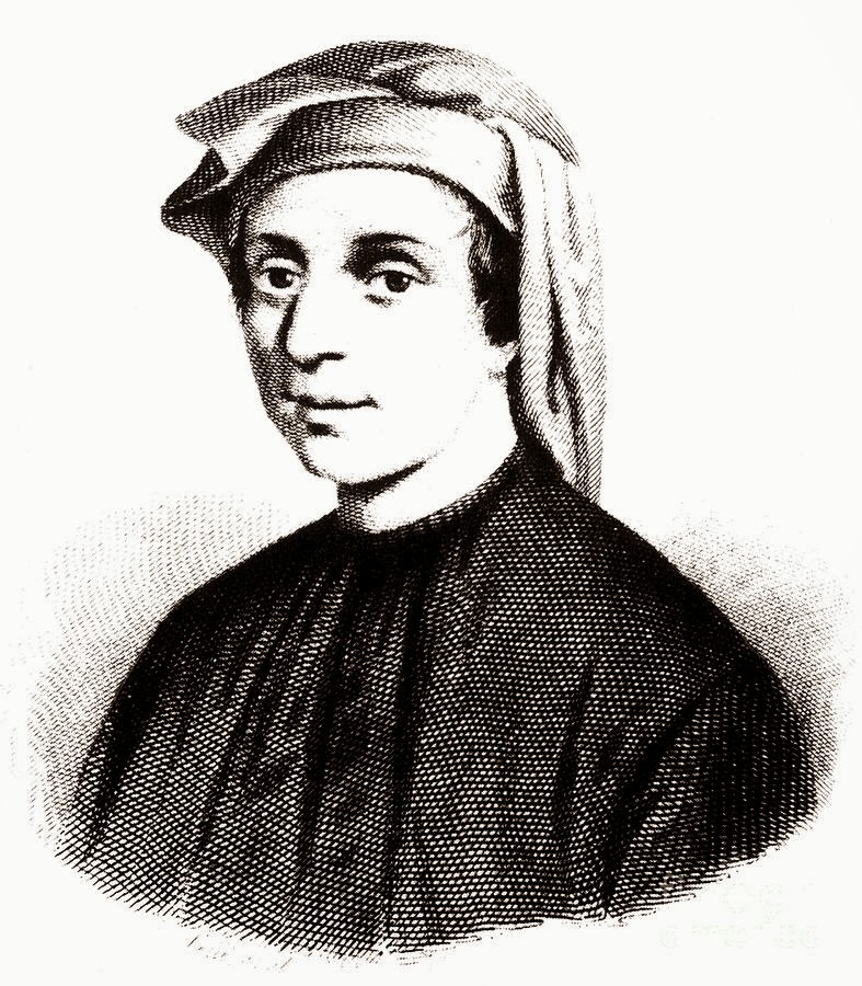
A man put one pair of rabbits in a certain place entirely surrounded by a wall. How many pairs of rabbits can be produced from that pair in a year, if the nature of these rabbits is such that every month each pair bears a new pair which from the second month on becomes productive?
Quote: Leonardo da Pisa, Liber Abaci (1202), translated by L. E. Sigler (Springer, 2002), pp. 404–405. Retrospective portrait from I benefattori dell’umanità, vol. VI (1850), public domain.
fib10 sequence you creared beforediff()) between successive numbers$A
[1] 3.141593
$B
[1] 0 1
$C
[1] 1 2 3 4 5 6 7 8 9 10
$D
[1] "one" "two"
List of 4
$ A: num 3.14
$ B: num [1:2] 0 1
$ C: int [1:10] 1 2 3 4 5 6 7 8 9 10
$ D: chr [1:2] "one" "two"
[1] 3.141593
$A
[1] 3.141593
List of 1
$ A: num 3.14
[1] 3.141593
Data frames are rectangular structures that are often used in data analysis
There is a built-in function called data.frame, but we recommend tibble, which is part of the dplyr package
You can look up the documentation of any R function this way: ?dplyr::tibble. If the package is loaded by using library(dplyr) you can omit dplyr:: prefix
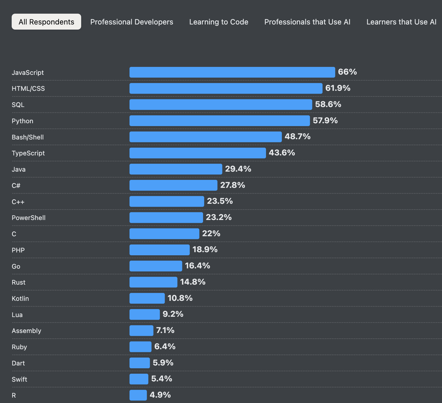
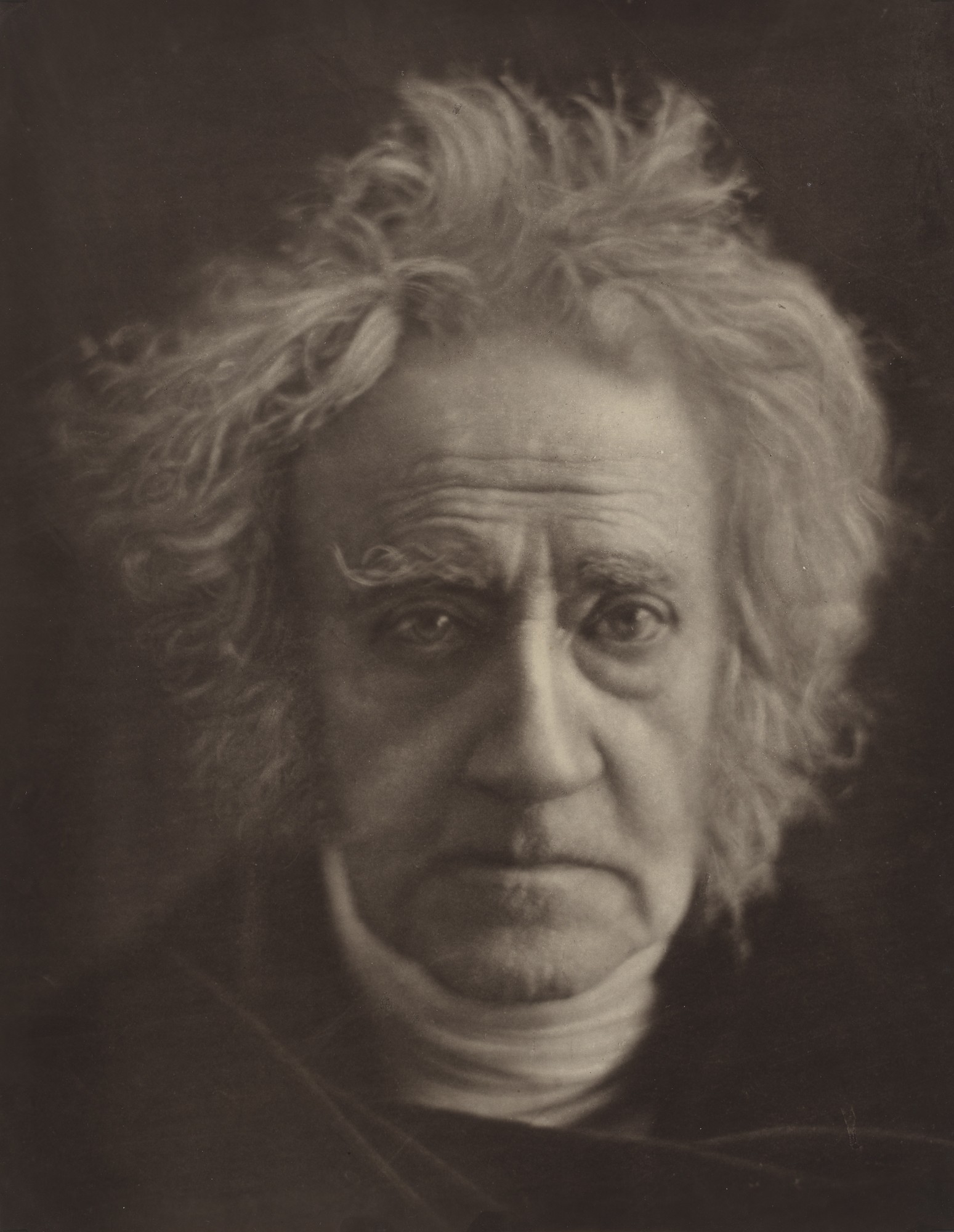
John F. W. Herschel’s data on the orbit of the Twin Stars \(\gamma\) Virginis
[1] "data.frame"
# A tibble: 14 × 4
year posangle distance velocity
<int> <dbl> <dbl> <dbl>
1 1720 160 17.2 -0.32
2 1730 157. 16.8 -0.354
3 1740 153 16.3 -0.376
4 1750 149. 15.5 -0.416
5 1760 144. 14.5 -0.478
6 1770 140. 13.7 -0.533
7 1780 134. 13.5 -0.547
8 1790 129. 12.9 -0.597
9 1800 122. 12.6 -0.632
10 1810 116. 11.2 -0.8
11 1815 111. 10.4 -0.929
12 1820 106. 9.57 -1.09
13 1825 98.3 7.09 -1.99
14 1830 84.3 4.9 -4.16
[1] "tbl_df" "tbl" "data.frame"
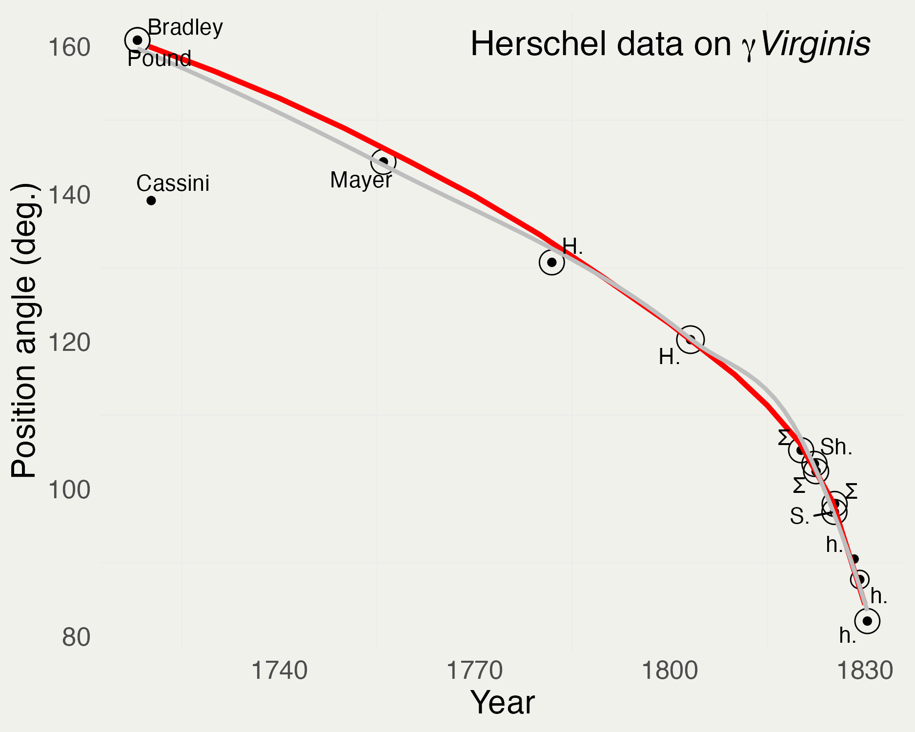
Code for generated the above plot can be found here.
Virginis.interp in a new tibble called virginis using as_tibble() functionvirginis$ like this: dataframe_name$variable_name
ggplot2 implements a grammar of graphics for building plots from data
Start with data and aesthetic mappings, then add geometric layers with +
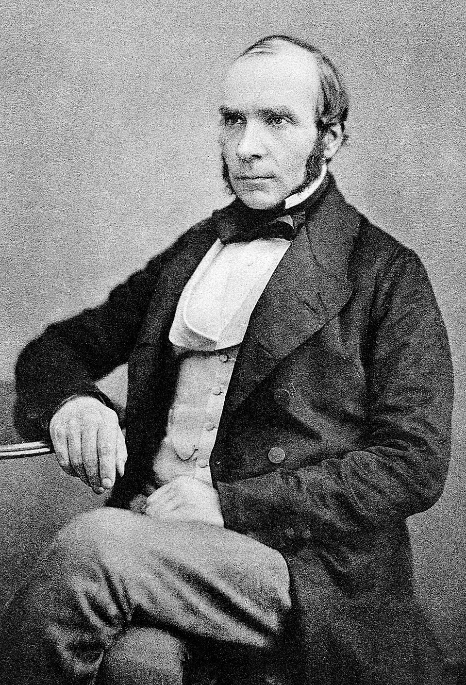
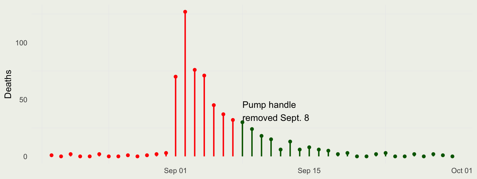
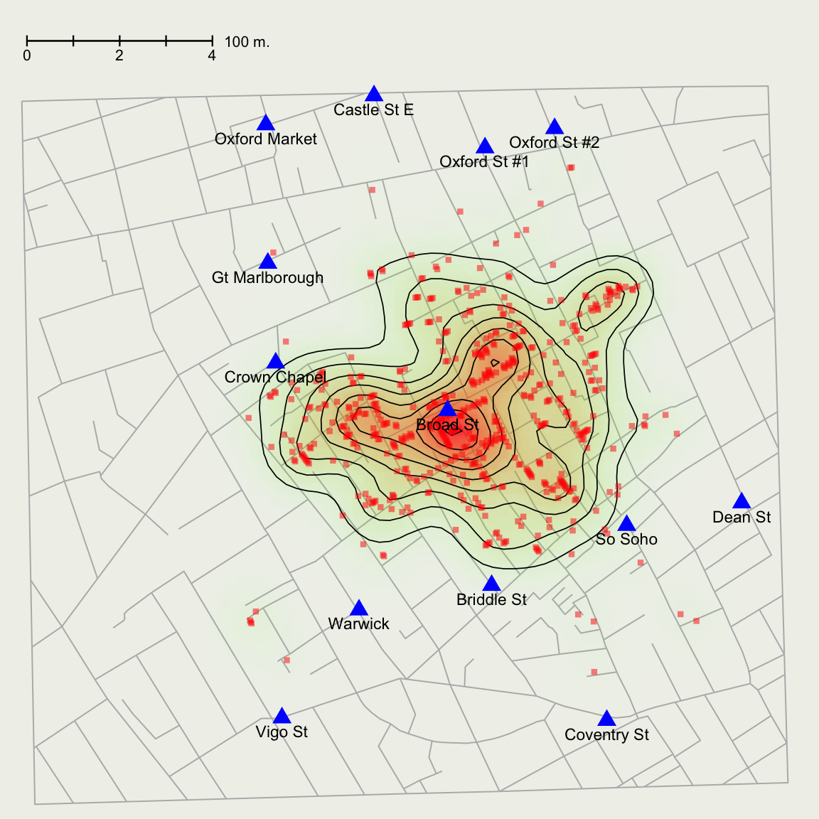
We will demonstrate with John Snow’s data from the 1854 cholera outbreak
library(HistData)
library(lubridate)
library(ggplot2)
library(dplyr)
# identify dates before and after the pump handle was removed
snow_dates <- Snow.dates |>
mutate(period = if_else(
date < mdy("09/08/1854"), "Before Sept. 8", "Sept. 8 onward"
))
ggplot(snow_dates, aes(x = date, y = deaths, color = period)) +
geom_linerange(aes(ymin = 0, ymax = deaths), linewidth = 0.8) +
geom_point(size = 1.5) +
annotate(
"text", x = mdy("09/08/1854"), y = 40,
label = "Pump handle\nremoved Sept. 8", hjust = 0
) +
scale_color_manual(
values = c("Before Sept. 8" = "red", "Sept. 8 onward" = "darkgreen"),
guide = "none"
) + labs(x = NULL, y = "Deaths")
We can learn a lot through simulation. We will start with the sample() function.
sample(x, size, replace = FALSE, prob = NULL)
[1] "H" "T" "T" "H" "T" "T" "H" "H" "H" "T"
[1] "T" "H" "H" "T" "T" "H" "H" "T" "H" "H"
[1] 1 0 1 1 1 0 0 1 1 1
sum() function or the formulahelp(if) statement and modulo operator help(%%); write a test to check your workest_prop contain?plot(), but we will do it with ggplotlibrary(ggplot2)
library(gridExtra)
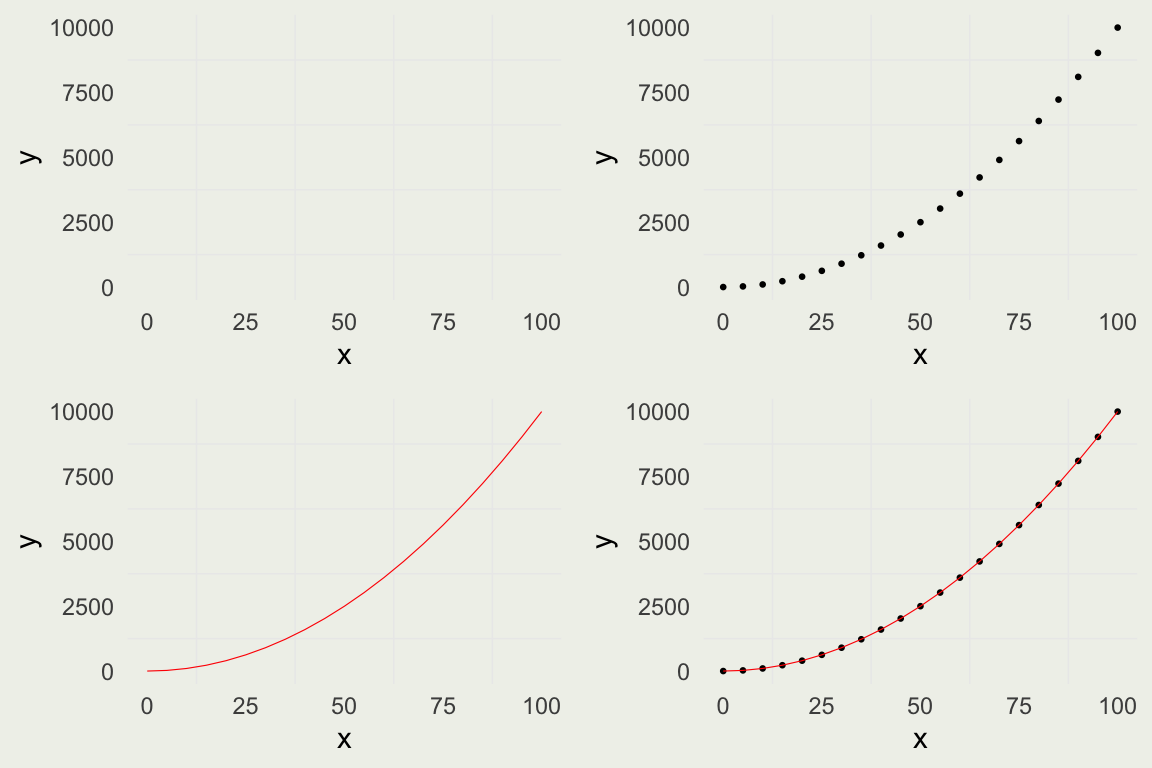
x <- seq(0, 100, by = 5)
y <- x^2
quadratic <- tibble(x = x, y = y)
p1 <- ggplot(data = quadratic,
mapping = aes(x = x, y = y))
p2 <- p1 + geom_point(size = 0.5)
p3 <- p1 + geom_line(linewidth = 0.2,
color = 'red')
p4 <- p1 + geom_point(size = 0.5) +
geom_line(linewidth = 0.2, color = 'red')
grid.arrange(p1, p2, p3, p4, nrow = 2)
set.seed(1)
n <- 1e4
est_prop <- numeric(n)
for (i in 1:n) {
x <- sample(coin, i, replace = TRUE)
est_prop[i] <- mean(x)
}
library(scales)
data <- tibble(num_flips = 1:n, est_prop = est_prop)
p <- ggplot(data = data, mapping = aes(x = num_flips, y = est_prop))
p + geom_line(size = 0.1) +
geom_hline(yintercept = 0.5, size = 0.2, color = 'red') +
scale_x_continuous(trans = 'log10', label = comma) +
xlab("Number of flips on Log10 scale") +
ylab("Estimated proportion of Heads") +
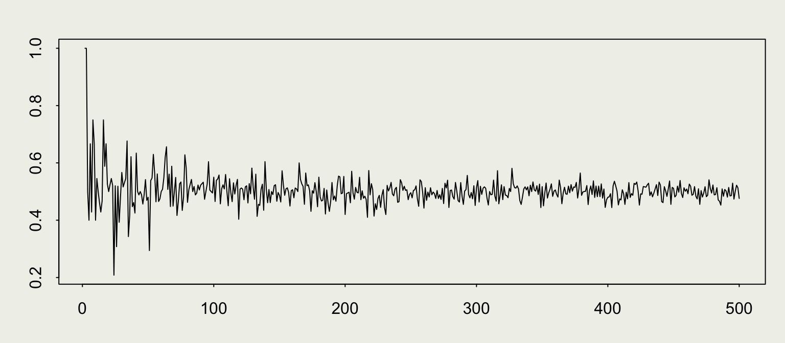
ggtitle("Error decreases with the size of the sample")We can see some evidence for the Law of Large Numbers.
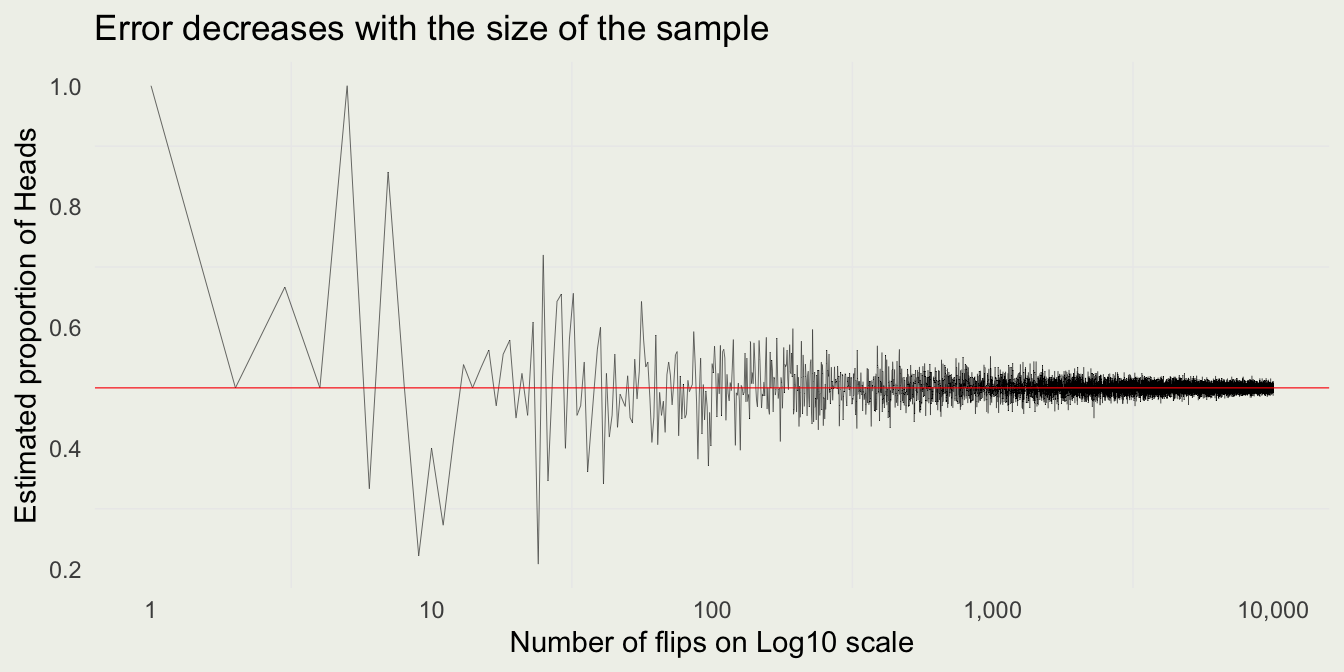
WLLN: \(\lim_{n \to \infty} \mathbb{P}\left( \left| \overline{X}_n - \mu \right| \geq \epsilon \right) = 0\)
Functions help you break up the code into self-contained, understandable pieces.
Functions take in arguments and return results. You saw functions like sum() and mean() before. Here, you will learn how to write your own.
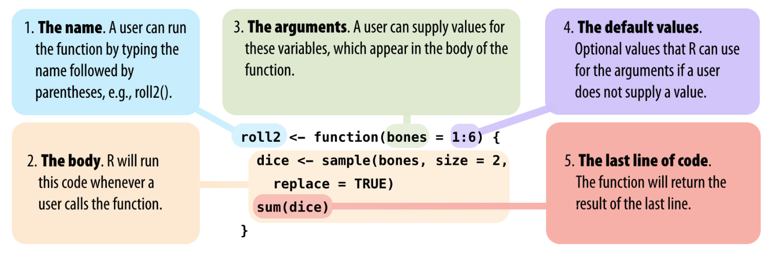
Source: Hands-On Programming with R
We will write a function that produces one estimate of the proportion given a fixed sample size n.
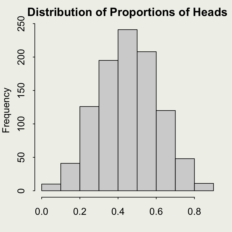
To reproduce our earlier example, generating estimates for increasing sample sizes, use map_dbl() function from purrr package. More on that here.
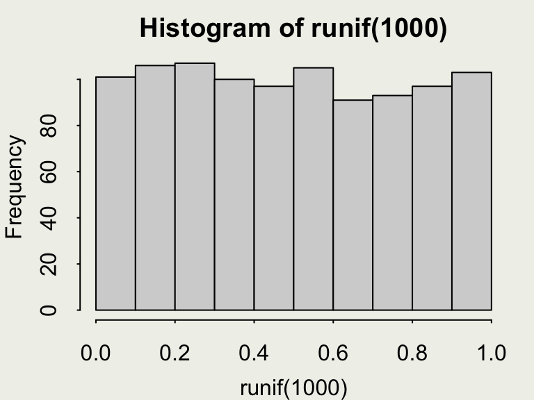
sample() function: runif(n, min = 0, max = 1)runif generates realizations of a random variable uniformly distributed between min and max.
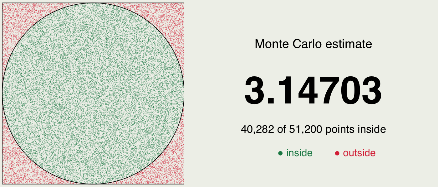
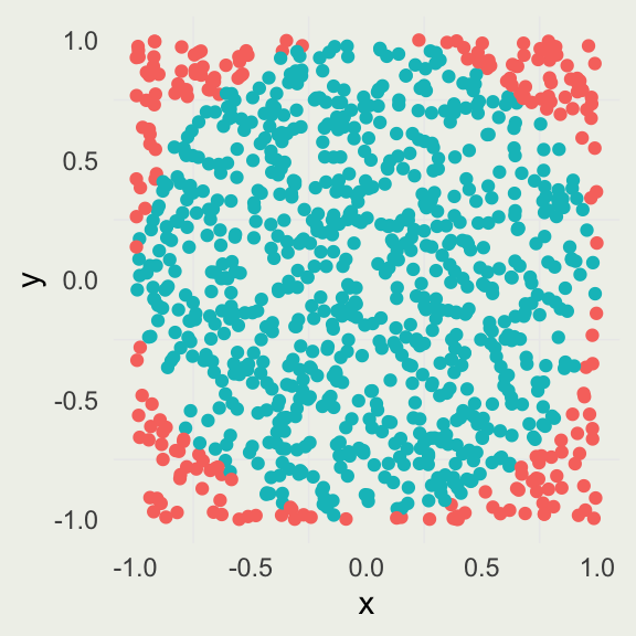
mean(runif(1e3, min = -1, max = 0))? Guess before running it.The idea is that we can approximate the ratio of the area of an inscribed circle, \(A_c\), to the area of the square, \(A_s\), by uniformly “throwing darts” at the square with the side \(2r\) and counting how many darts land inside the circle versus inside the square.
\[ \begin{align} A_{c}& = \pi r^2 \\ A_{s}& = (2r)^2 = 4r^2 \\ \frac{A_{c}}{A_{s}}& = \frac{\pi r^2}{4r^2} = \frac{\pi}{4} \implies \pi = \frac{4A_{c}}{A_{s}} \end{align} \]
To estimate \(\pi\), we perform the following simulation:
\[ \begin{align} X& \sim \text{Uniform}(-1, 1) \\ Y& \sim \text{Uniform}(-1, 1) \\ \pi& \approx \frac{4 \sum_{i=1}^{N} \I(x_i^2 + y_i^2 < 1)}{N} \end{align} \]
The numerator is a sum over an indicator function \(\I\), which evaluates to \(1\) if the inequality holds and \(0\) otherwise.
viewof n = {
const form = html`<form style="display: flex; align-items: center; justify-content: flex-start; gap: 0.8rem; width: 780px; max-width: 100%; box-sizing: border-box; padding-left: 8px; margin: 0.2rem auto 0.7rem;">
<label for="pi-draws" style="font-size: 0.65em; white-space: nowrap;">Number of draws, <i>n</i></label>
<input id="pi-draws" type="range" min="0" max="10" step="1" value="3" style="flex: 1; min-width: 0;">
<output style="font-size: 0.65em; min-width: 5.5em; text-align: left;"></output>
</form>`;
const slider = form.querySelector("input");
const output = form.querySelector("output");
const update = () => {
form.value = 100 * 2 ** Number(slider.value);
output.value = form.value.toLocaleString();
};
slider.addEventListener("input", update);
update();
return form;
}
piSimulation = {
const size = 320;
const padding = 8;
const span = size - 2 * padding;
const pixelRatio = window.devicePixelRatio || 1;
const canvas = DOM.canvas(size * pixelRatio, size * pixelRatio);
canvas.style.width = `${size}px`;
canvas.style.height = `${size}px`;
const context = canvas.getContext("2d");
context.scale(pixelRatio, pixelRatio);
context.fillStyle = "#ffffff";
context.fillRect(padding, padding, span, span);
let inside = 0;
const dotSize = n <= 5000 ? 2 : 1;
for (let i = 0; i < n; i++) {
const x = 2 * Math.random() - 1;
const y = 2 * Math.random() - 1;
const isInside = x * x + y * y < 1;
inside += isInside;
context.fillStyle = isInside
? "rgba(25, 135, 84, 0.65)"
: "rgba(220, 53, 69, 0.65)";
context.fillRect(
padding + (x + 1) * span / 2,
padding + (1 - y) * span / 2,
dotSize,
dotSize
);
}
context.strokeStyle = "#222222";
context.lineWidth = 1;
context.strokeRect(padding, padding, span, span);
context.beginPath();
context.arc(size / 2, size / 2, span / 2, 0, 2 * Math.PI);
context.stroke();
const estimate = 4 * inside / n;
return html`<div style="display: grid; grid-template-columns: 340px 1fr; align-items: center; gap: 1.4rem; max-width: 780px; margin: 0 auto;">
<div>${canvas}</div>
<div style="text-align: center;">
<div style="font-size: 0.65em;">Monte Carlo estimate</div>
<div style="font-size: 2.2em; font-weight: 600; line-height: 1.15;">${estimate.toFixed(5)}</div>
<div style="font-size: 0.55em; margin-top: 0.4rem;">${inside.toLocaleString()} of ${n.toLocaleString()} points inside</div>
<div style="font-size: 0.5em; margin-top: 0.5rem;"><span style="color: #198754;">● inside</span> <span style="color: #dc3545;">● outside</span></div>
</div>
</div>`;
}