SMaC: Statistics, Math, and Computing (Read)

APSTA-GE 2006: Applied Statistics for Social Science Research

Eric.Novik@nyu.edu | Summer 2026 | Session 2

Session 2 Outline

  • Linear, exponential, and logarithmic functions

  • Limits

  • Definition of the derivative

  • Rules of differentiation

  • The chain rule and product rule

Lines

  • We typically use the slope-intercept form of the line: \(y = a + bx\), where \(a = y(0)\) is the intercept and \(b = \Delta y / \Delta x\) is the slope (rise over run).
  • For example: \(y = 1.5 + 0.5x\).
  • If \(b = 0\), the line is horizontal.

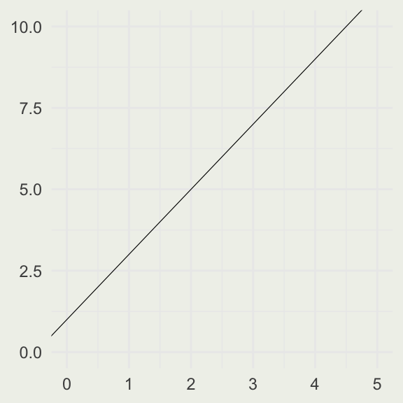
A graph of a line with the equation \(y = 1 + 2x\).

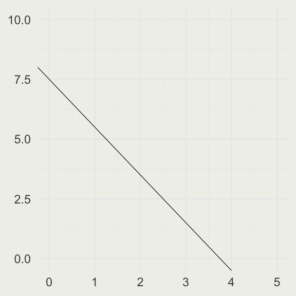
A graph of a line with the equation \(y = 7.5 - 2x\).

# y = 1 + 2x
p <- ggplot() + xlim(0, 5) + ylim(0, 10)
p + geom_abline(slope = 2, intercept = 1, linewidth = 0.2)

# y = 7.5 - 2x
p <- ggplot() + xlim(0, 5) + ylim(0, 10)
p + geom_abline(slope = -2, intercept = 7.5, linewidth = 0.2)

# to see some other ways of plotting lines
?geom_abline

Your Turn

  • Turn the following code into a function called plot_line(slope, intercept)
  • Test it for different values of slope and intercept
p <- ggplot() + xlim(0, 5) + ylim(0, 10)
p + geom_abline(slope = 2, intercept = 1, linewidth = 0.2)

Choose test values whose lines are visible in the fixed plotting window.

Exponential Functions

  • The idea of an exponential function is that the rate of change of the function at time \(t\) is proportional to the value of the function at time \(t\). In other words:

\[ \frac{\text{d}[y(t)]}{\text{d}t} = k \cdot y(t) \]

  • The general solution to this differential equation is \(y(t) = C e^{kt}\), where \(C = y(0)\).

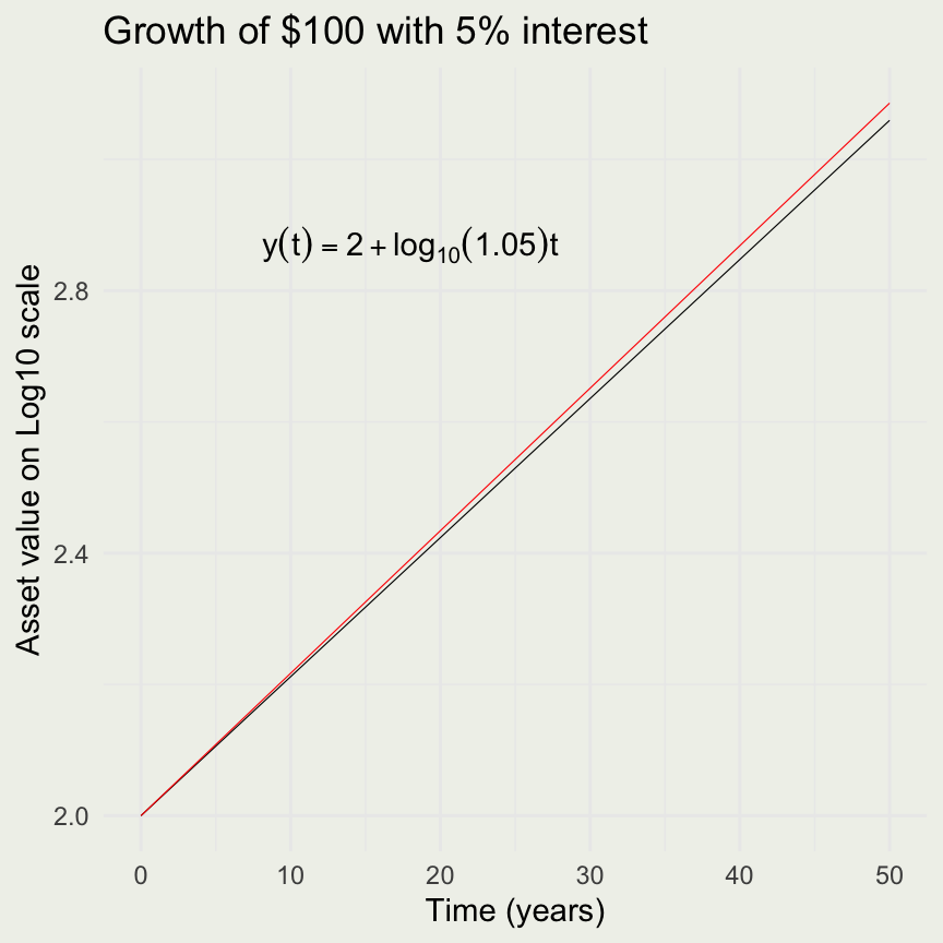
  • Think of population growth or growth of an interest-bearing asset.

Example: Compound Interest

An asset that has a value \(A\) is invested with an annual interest rate \(r\). What is the balance in the account, \(P_1\), at the end of the first year?

\[ P_1 = A + rA = A(1 + r) \]

After year two, the value is:

\[ P_2 = P_1 + rP_1 = P_1(1 + r) = \\ A(1 + r)(1 + r) = A(1 + r)^2 \]

And after year \(t\), the value is:

\[ P(t) = A(1 + r)^t \]

What if we compound the interest twice per year? In that case:

\[ P_1 = A \left (1 + \frac{r}{2} \right)^2 \]

If we compound \(n\) times per year, the balance after one year would be:

\[ P_n(1) = A \left (1 + \frac{r}{n} \right)^n \]

Combining these ideas, if we compound \(n\) times per year, for \(t\) years, we get:

\[ P_n(t) = A \left (1 + \frac{r}{n} \right)^{nt} \]

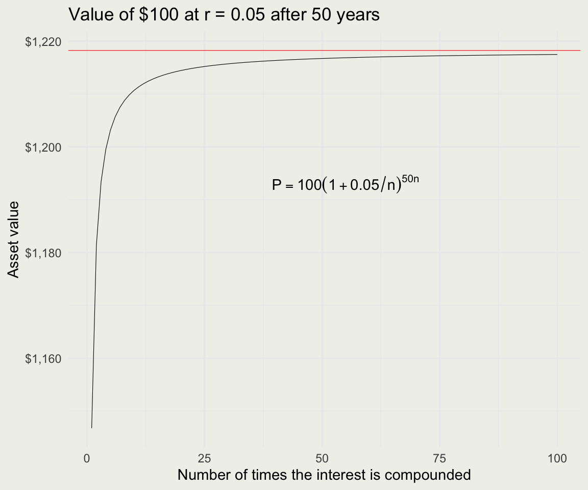
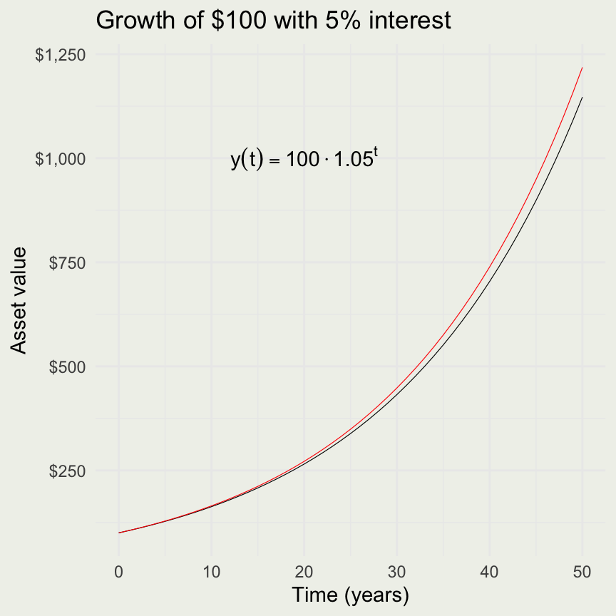
Letting \(n \to \infty\) gives continuous compounding. Both the finite- and continuous-compounding formulas are exponential functions of time.

Example: Compound Interest

rate <- 0.05    # interest rate r
P <- 100        # principal P
n_comp <- 1:100 # number of compoundings n

Pn <- function(n, A, r, t) A * (1 + r/n)^(t*n)
Pe <- function(A, r, t) A * exp(r * t)

pn <- Pn(n = n_comp, A = P, r = rate, t = 50)
pe <- Pe(A = P, r = rate, t = 50)

d <- data.frame(n_comp, pn)
p <- ggplot(d, aes(n_comp, pn))
p + geom_line(linewidth = 0.2) +
  geom_hline(yintercept = pe, color = 'red', linewidth = 0.2) +
  xlab("Number of times the interest is compounded") +
  ylab("Value of an asset") +
  ggtitle("Value of $100 at r = 0.05 after 50 years") 

Your Turn

Suppose a particular population of bacteria is known to double in size every 4 hours. If a culture starts with 1000 bacteria, what is the population after 10 hours and 24 hours?

The Number \(e\)

  • Recall the equation for asset value after \(t\) years compounded \(n\) times:

\[ P_n(t) = A \left (1 + \frac{r}{n} \right)^{nt} \]

  • Let \(m = n/r\) and take the limit as \(m \to \infty\).

\[ P_\infty(t) = A \lim_{m \to \infty} \left ( 1 + \frac{1}{m} \right)^{m(rt)} \]

The Number \(e\)

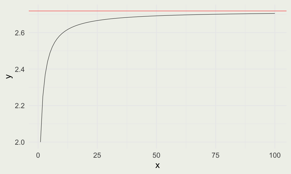
  • We can compute the value of \(\left ( 1 + \frac{1}{m} \right)^m\) as m increases.

  • The number that this limit approaches is called \(e\).

\[ P_\infty(t) = A \lim_{m \to \infty} \left ( 1 + \frac{1}{m} \right)^{m(rt)} = A e^{rt} \]

f <- function(m) (1 + 1/m)^m
x <- 1:100
y <- f(x)
p <- ggplot(data.frame(x, y), aes(x, y))
p + geom_line(linewidth = 0.2) +
  geom_hline(yintercept = exp(1), color = 'red', linewidth = 0.2)

Properties of Exponents

  • \(a^x a^y = a^{x + y}\)
2^7 * 2^8 == 2^(7 + 8) 
[1] TRUE
  • \(\frac{a^x}{a^y} = a^{x-y}\)
2^7 / 2^8 == 2^(7 - 8) 
[1] TRUE
  • \((a^x)^y = a^{xy}\)
(2^7)^8 == 2^(7*8)
[1] TRUE
  • \((ab)^x = a^x b^x\)
(2*3)^7 == 2^7 * 3^7
[1] TRUE
  • \(\frac{a^x}{b^x} = \left( \frac{a}{b} \right)^x\)
isTRUE(all.equal(2^4 / 3^4, (2/3)^4))
[1] TRUE

Your Turn

Suppose $750 is invested in an account at an annual interest rate of 5.5%, compounded continuously. Let \(t\) denote the number of years after the initial investment and \(A(t)\) denote the amount of money in the account at time \(t\). Find a formula for \(A(t)\). Find the amount of money in the account after 5 years, 10 years, and 50 years.

Logarithmic functions

  • For \(a > 0\) and \(a \ne 1\), an exponential function of the form \(f(x) = a^x\) is one-to-one, so it has an inverse called a logarithmic function. Logarithm arguments must be positive.

  • In R and this course, \(\log\) means the natural log, base \(e\). For a log-scale coefficient \(\beta\), the exact percentage change is \(100(e^\beta - 1)\%\); \(100\beta\%\) is a useful approximation only when \(\beta\) is small. For example, \(\log(1.04) \approx 0.0392\).

  • The following relationship always holds for \(a > 0\): \(a^t = e^{\log(a)t}\) since \(e^{\log(a)} = a\)

  • \(\log_a(uv) = \log_a(u) + \log_a(v)\)

  • \(\log_a(u/v) = \log_a(u) - \log_a(v)\)

  • \(\log_a u^n = n \log_a u\)

In statistics and machine learning, we often want to normalize a vector so its components add to one. The softmax function is

\[ \operatorname{softmax}(x)_i = \frac{\exp(x_i)}{\sum_{j=1}^N \exp(x_j)}. \]

If \(x\) has length 3, the numerator is a length-3 vector, the denominator is a scalar, and the resulting length-3 vector adds to 1.

softmax_unsafe <- function(x) exp(x) / sum(exp(x))

y_small <- 1:3
softmax_unsafe(y_small)
[1] 0.09003057 0.24472847 0.66524096
y_large <- c(1e3, 1e3 + 1, 1e3 + 2)
exp(y_large)
[1] Inf Inf Inf
softmax_unsafe(y_large)
[1] NaN NaN NaN

The large inputs overflow: their exponentials are too large for the computer to represent directly.

We can instead work on the log scale:

\[ \log \operatorname{softmax}(x)_i = x_i - \log \sum_{j=1}^N \exp(x_j). \]

The second term is the log-sum-exp, or LSE. To evaluate it stably, subtract the largest input before exponentiating.

\[ \begin{aligned} m &= \max_j x_j, \\ \operatorname{LSE}(x) &= \log \sum_{j=1}^N \exp(x_j) \\ &= m + \log \sum_{j=1}^N \exp(x_j - m). \end{aligned} \]

Because \(m = \max_j x_j\), the largest shifted exponent is zero and every other shifted exponent is negative.

Your Turn: write LSE(x) and log_softmax(x), test them on small and large inputs, exponentiate the log probabilities, and check that they add to 1.

LSE <- function(x) {
  m <- max(x)
  m + log(sum(exp(x - m)))
}

log_softmax <- function(x) x - LSE(x)
softmax <- function(x) exp(log_softmax(x))

softmax(y_small)
[1] 0.09003057 0.24472847 0.66524096
softmax(y_large)
[1] 0.09003057 0.24472847 0.66524096
sum(softmax(y_large))
[1] 1

Limits

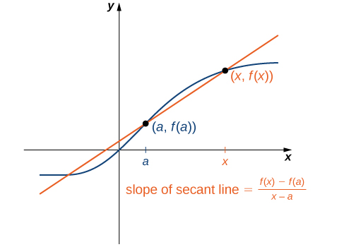
A limit is the value a function approaches as its input gets arbitrarily close to a specified point. The limit can exist even when the function is undefined there or has a different value there.

This demo shows what happens to the secant line as it approaches the tangent.

A Cruel Joke

A thousand years from now, your friends drug you, load you onto a ship, and fire it at the Moon. You wake in a spacesuit on the surface: a ship, a 100 m tower beside you, a metal ball stamped 1 kg, and a stopwatch.

  • The ship’s autopilot has the equations of motion programmed in — but it is missing one number: the Moon’s gravitational acceleration \(g\)

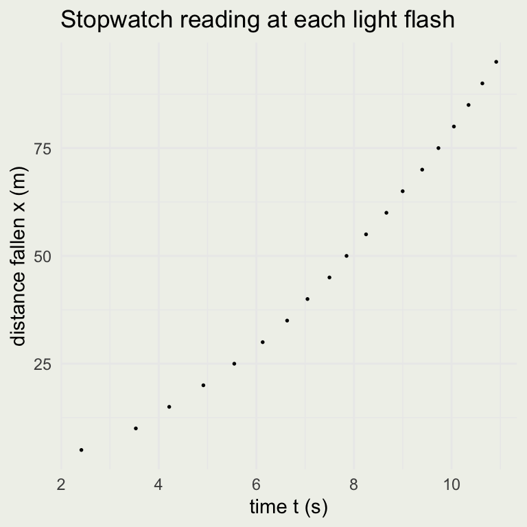
  • Your plan: climb the tower, drop the ball, and record the time it passes each red mark (spaced 5 m apart, 20 marks down)

  • Each mark has a sensor: as the ball passes, it flashes a light, so from the top you read the time off your stopwatch at each flash

  • From those \((t_k, x_k)\) pairs you will infer \(g\) — and fly home

Setting Up the Equation of Motion

  • Let \(x\) measure downward distance from the release point, so downward is positive. There is no atmosphere on the Moon, so the only force on the ball is gravity. Newton’s second law gives:

\[ m\,\ddot{x} = m\,g \quad\Rightarrow\quad \ddot{x} = g \]

  • The mass cancels — that is why the 1 kg label is a red herring. This is Galileo’s insight, confirmed on the Moon by Apollo 15’s hammer-and-feather drop.

  • Integrating twice (we cover integration in Session 3), and dropping from rest, gives the solution we will use:

\[ v(t) = g\,t, \qquad x(t) = \tfrac{1}{2}\, g\, t^2 \]

  • So the acceleration is the second derivative of position — a constant \(g\) — which is exactly the unknown the mission needs.

The Drop, in Data

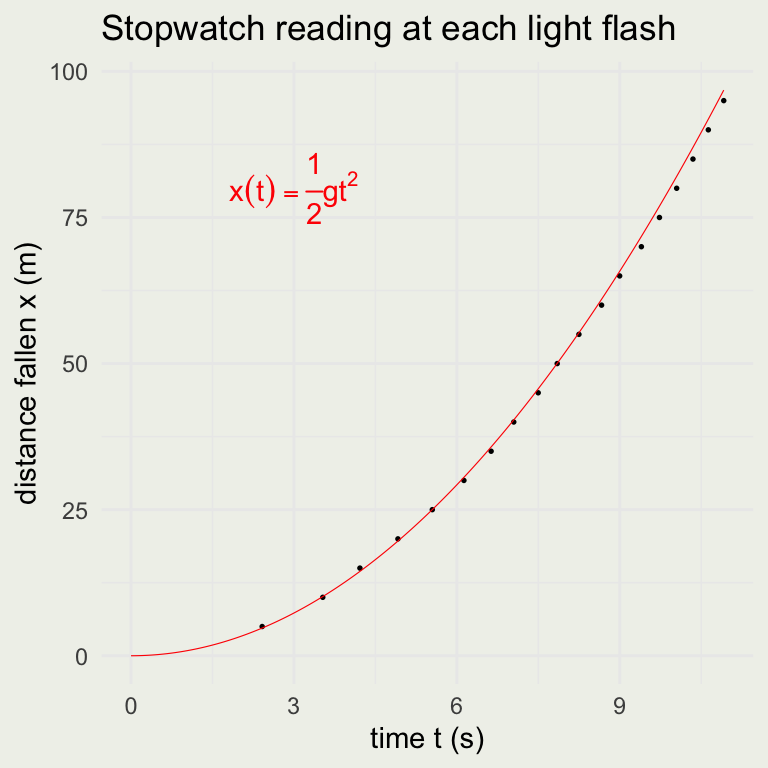
Low gravity is a feature: on the Moon a 100 m drop takes about 11 s, slow enough to read marks with a stopwatch. On Earth it would take 4.5 s.

The inference problem (Session 6) is to recover \(g\) from noisy time readings at the known sensor positions, assuming \(x(t) = \tfrac{1}{2} g t^2\). The curve below uses the accepted reference value \(g_{\mathrm{ref}} = 1.625\ \text{m/s}^2\); it is not an estimate from these observations.

Oxygen is limited, so each drop costs you. One drop gives up to 20 timed marks (this run caught 19) — how many marks, and how many drops, do we need to pin down \(g\) to one decimal place? To two? We return to this in Session 7.

Average Velocity and the Secant

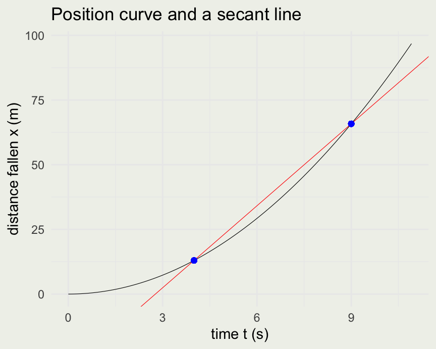
Before we can find \(g\), we need to understand velocity. What was the ball’s average velocity between \(t_1\) and \(t_2\) seconds? This is the slope of the secant line:

\[ \bar{v} = \frac{\Delta x}{\Delta t} = \frac{x(t_2) - x(t_1)}{t_2 - t_1} = \frac{\tfrac{1}{2} g\, t_2^2 - \tfrac{1}{2} g\, t_1^2}{t_2 - t_1} = \tfrac{1}{2} g\, (t_1 + t_2) \]

t1 <- 4; t2 <- 9
x1 <- 0.5 * g_ref * t1^2; x2 <- 0.5 * g_ref * t2^2
slope <- (x2 - x1) / (t2 - t1)            # avg velocity = ½ g (t1 + t2)
ggplot(sol, aes(t, x)) + geom_line(linewidth = 0.2) +
  geom_abline(slope = slope, intercept = x1 - slope * t1,
              color = 'red', linewidth = 0.2) +
  geom_point(aes(x = t1, y = x1), color = 'blue') +
  geom_point(aes(x = t2, y = x2), color = 'blue') +
  xlab("time t (s)") + ylab("distance fallen x (m)") +
  ggtitle("Position curve and a secant line")

What if we wanted the speedometer reading at an instant \(t\), not the average over an interval? This is where the limit comes in.

\[ v = \lim_{\Delta t \to 0} \frac{\Delta x}{\Delta t} = \frac{dx}{dt} \]

The Derivative

  • How do we compute this limit, which we wrote as \(dx/dt\)?

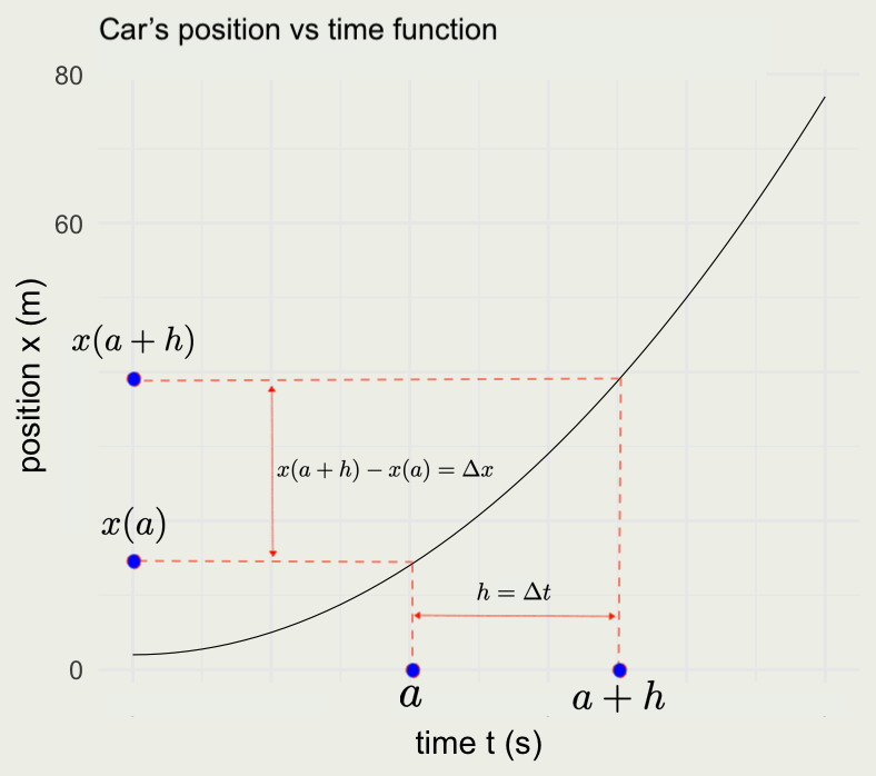
  • We re-write the secant or average velocity equation in the following way:

\[ \begin{eqnarray} \bar v & = & \frac{x(a + h) - x(a)}{a + h - a} = \frac{x(a + h) - x(a)}{h} \\ v & = & \lim_{h \to 0} \frac{x(a + h) - x(a)}{h} \\ \end{eqnarray} \]

The Derivative

  • Our problem is to find the velocity at time \(t\) given the position function \(x(t) = \tfrac{1}{2} g t^2\).

\[ \begin{eqnarray} v & = & \lim_{h \to 0} \frac{x(t + h) - x(t)}{h} = \lim_{h \to 0} \frac{\tfrac{1}{2} g (t + h)^2 - \tfrac{1}{2} g t^2}{h} = \\ & \lim_{h \to 0} & \frac{g t h + \tfrac{1}{2} g h^2}{h} = \lim_{h \to 0} \left(g t + \tfrac{1}{2} g h\right) = g t \end{eqnarray} \]

  • Using the accepted value \(g \approx 1.62\ \text{m/s}^2\), the speedometer at \(t = 4\) reads \(1.62 \cdot 4 \approx 6.5\ \text{m/s}\) downward.

  • The velocity is the derivative of position with respect to time, and we can write:

\[ v(t) = \frac{dx}{dt} = g t \]

The Derivative

  • But what about acceleration?
  • Acceleration is a change in velocity with respect to time or the second derivative of position:

\[ a(t) = \frac{dv}{dt} = \frac{d}{dt} \left( \frac{d x}{d t} \right) = \frac{d^2 x}{d t^2} \]

  • We take the limit again, this time of the velocity function \(v(t) = g t\):

\[ a = \frac{dv}{dt} = \lim_{h \to 0} \frac{g(t + h) - g t}{h} = \lim_{h \to 0} \frac{g h}{h} = \lim_{h \to 0} g = g \]

  • The acceleration \(a(t) = g\) does not depend on \(t\) — it is constant. This constant is exactly what the mission needs. Recovering it from the drop data is the inference problem we solve in Sessions 6 and 7.
  • It would be cumbersome to compute derivatives this way. Fortunately, we have shortcuts.

Rules of Differentiation

  • We will state a few rules of differentiation without deriving them

\[ \begin{eqnarray} \frac{d}{dx}(c) & = & 0 \\ \frac{d}{dx}(x) & = & 1 \\ \frac{d}{dx}(x^n) & = & n x^{n-1} \\ \frac{d}{dx}[c f(x)] & = & c \frac{d}{dx}[f(x)] \\ \frac{d}{dx}[f(x) + g(x)] & = & \frac{d}{dx}f(x) + \frac{d}{dx}g(x) \\ \frac{d}{dx}(e^x) & = & e^x \\ \frac{d}{dx}\log(x) & = & \frac{1}{x} \end{eqnarray} \]

  • If you are interested in why the last statement is true, see this.

  • The derivatives of trigonometric functions can be found here.

Your Turn

  • Suppose that on a different moon a calibration drop (with a small initial push, so it is not released from rest) produced the position function:

\[ x(t) = 4 + 3t + 5t^2 \]

  • What is the ball’s position at time zero and time 1 second?

  • What is the velocity at time zero?

  • What is the velocity and acceleration at 5 seconds?

  • What is this moon’s gravitational acceleration \(g\)? (Hint: compare \(a(t)\) to \(\ddot{x} = g\).)

Product Rule and Chain Rule

  • Product and chain rules help us differentiate products and compositions of functions, respectively.
  • Intuition for them can be found in the Essence of Calculus video.
  • We will state them here without derivation.

\[ \frac{d}{dx}[f(x) g(x)] = f(x) \frac{d}{dx}[g(x)] + g(x)\frac{d}{dx}[f(x)] \]

  • If \(F = f \circ g\), in that \(F(x)= f(g(x))\):

\[ F'(x) = f'(g(x))g'(x) \]

Example of a Product Rule

  • Suppose we wanted to compute the derivative of \(x(t) = \sin(t) \cos(t)\)

\[ \begin{eqnarray} \frac{d}{dt}(\sin(t) \cos(t)) & = & \\ \sin(t)\frac{d}{dt}[\cos(t)] + \cos(t)\frac{d}{dt}[\sin(t)] & = & \\ \sin(t) (-\sin(t)) + \cos(t)\cos(t) & = & \\ \cos^2(t) - \sin^2(t) \end{eqnarray} \]

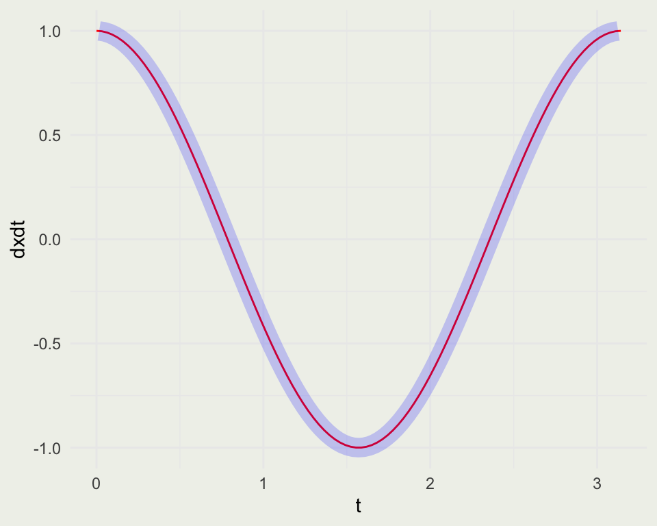
Approximating Derivatives

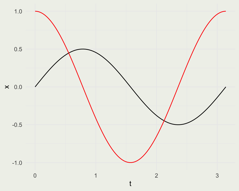
library(ggplot2)
library(dplyr)
n <- 100
t <- seq(0, pi, length.out = n)
x <- sin(t) * cos(t)
dxdt <- cos(t)^2 - sin(t)^2

d <- tibble(t, x, dxdt)
p <- ggplot(d, aes(t, x))
p + geom_line() + geom_line(aes(y = dxdt), color = "red")

# approximate the derivative on each interval and align it to the midpoint
appr <- tibble(
  t = (t[-1] + t[-n]) / 2,
  appr_dxdt = diff(x) / diff(t)
)

p + geom_line(aes(y = dxdt), color = "red") +
  geom_line(
    data = appr, aes(t, appr_dxdt),
    color = "blue", linewidth = 5, alpha = 1/5
  )

Examples of the Chain Rule

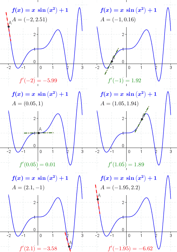
  • What is the derivative of \(\sin(x^2)\)? It is \(2x \cos(x^2)\)
  • Your turn: \[ \frac{d}{dx} \left( e^{x^2 \cos(x)} \right ) = \]

\[ e^{x^2 \cos(x)} \left(2x \cos(x) - x^2 \sin(x)\right) \]

Homework

  • A particle moves counter-clockwise in uniform circular motion, with \(R > 0\) and \(\omega > 0\):

\[ x(t) = R \cos(\omega t) \\ y(t) = R \sin(\omega t) \]

  • Here \(R\) is the radius, \(\omega\) is the angular frequency in radians per unit time, and the period is \(T = 2\pi / \omega\).
  • Create position functions that take \(R\), \(t\), and \(\omega\) as arguments.
  • Create a length-100 vector \(t\) covering one full rotation.
  • Plot \(x(t)\) and \(y(t)\) against \(t\) on the same graph, then plot \(y\) against \(x\). Explain the geometry.
  • Create four more functions: velocity and acceleration in the \(x\) and \(y\) directions.
  • Plot each velocity component with its corresponding position component, and each acceleration component with its corresponding position component.
  • Verify that \(\mathbf{a}(t) = -\omega^2 \mathbf{r}(t)\). Explain what the position, velocity, and acceleration vectors show.