SMaC: Statistics, Math, and Computing
APSTA-GE 2006: Applied Statistics for Social Science Research
Eric.Novik@nyu.edu | Summer 2026 | Session 2
Mission: recover lunar gravity
100 m tower · 20 flashes · 1 stopwatch
1 kg ball · unknown \(g\)
\[
(t_k, x_k) \longrightarrow \boxed{g} \longrightarrow \text{home}
\]
functions \(\rightarrow\) rates \(\rightarrow\) limits \(\rightarrow\) derivatives
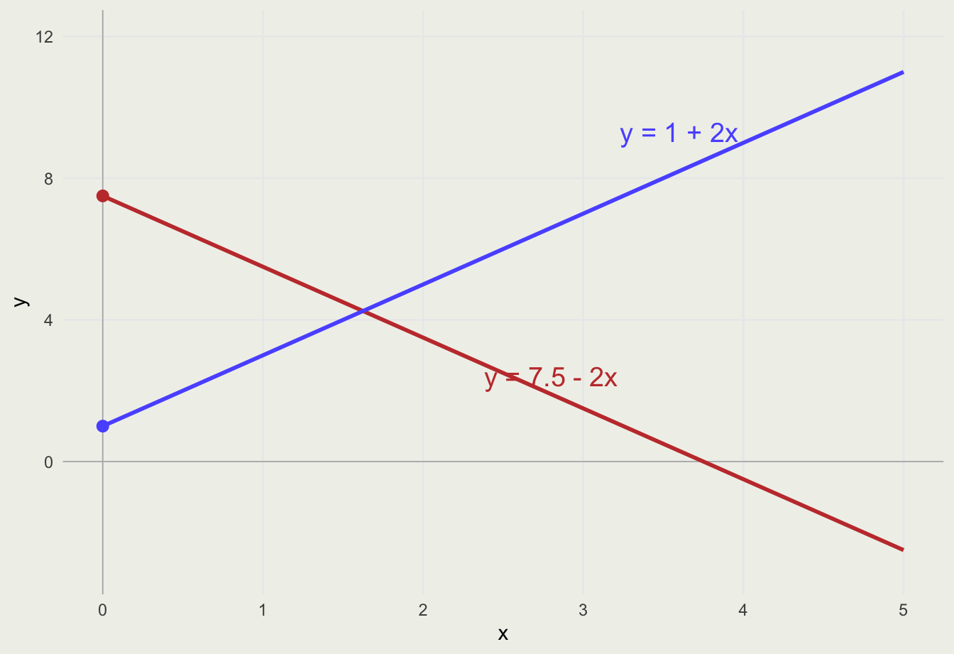
A line is a constant rate
\[a = y(0)\]
\[b = \frac{\Delta y}{\Delta x}\]
Your Turn: plot_line()
Write plot_line(slope, intercept).
plot_line <- function(slope, intercept) {
  x <- seq(0, 5, length.out = 100)
  # construct y
  # return a ggplot
}
Test three cases:
\[b > 0 \qquad b = 0 \qquad b < 0\]
Use values that remain visible for \(0 \le x \le 5\).
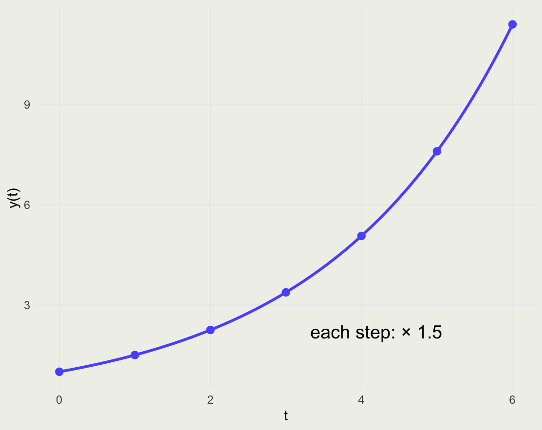
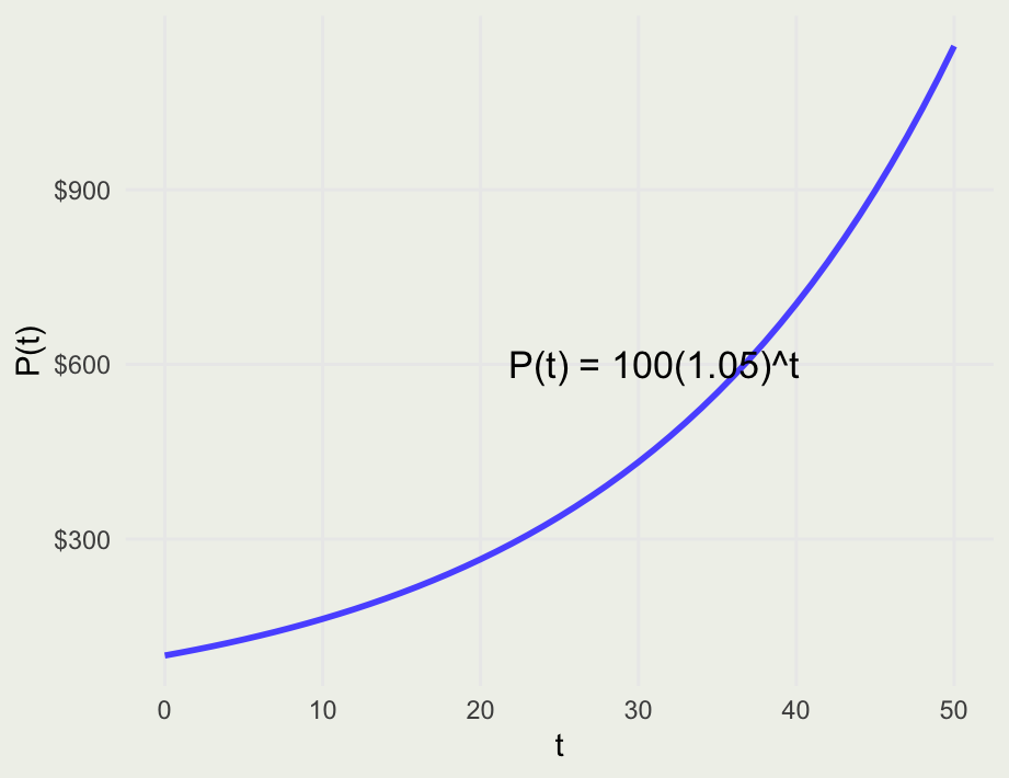
Exponential growth
\[
\frac{y(t + 1)}{y(t)} = b
\]
\[
y(t) = A b^t = A e^{kt},
\qquad k = \log b
\]
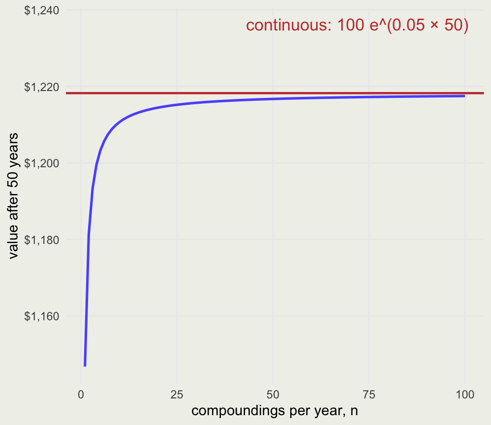
Compound interest
\[
A \longrightarrow A(1+r) \longrightarrow A(1+r)^2
\]
\[
P(t) = A(1+r)^t
\]
\[
P_n(t) = A\left(1 + \frac{r}{n}\right)^{nt}
\]
\[
P_\infty(t) = A e^{rt}
\]
Your Turn: bacterial growth
\(N(0) = 1000\) · doubles every 4 hours
\[
N(10) = \; ?
\qquad\qquad
N(24) = \; ?
\]
\[
N(t) = 1000 \cdot 2^{t/4}
\]
\[
N(10) \approx 5657
\qquad\qquad
N(24) = 64{,}000
\]
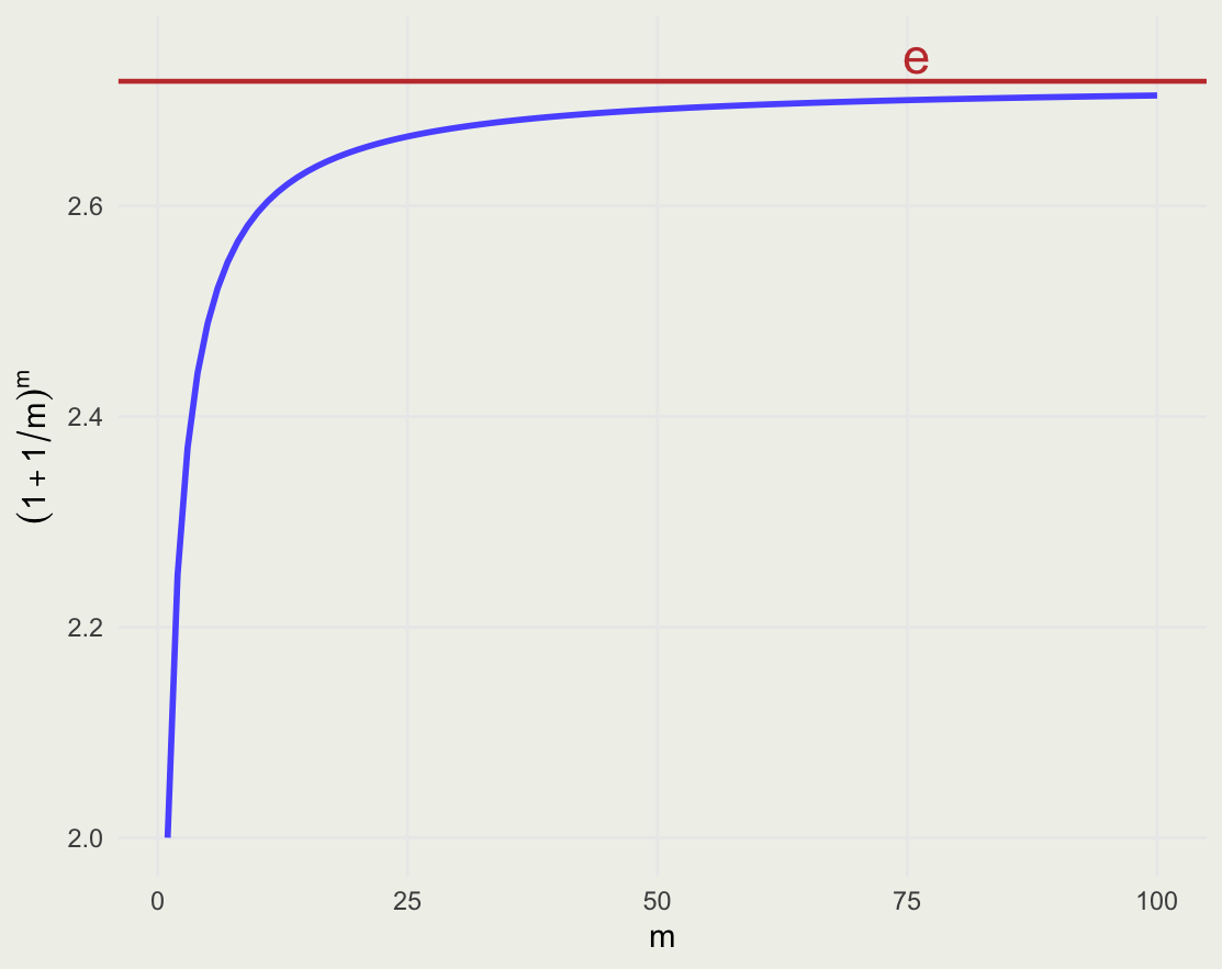
The limit that defines \(e\)
\[
e = \lim_{m \to \infty}
\left(1 + \frac{1}{m}\right)^m
\]
\[
\lim_{n \to \infty}
A\left(1 + \frac{r}{n}\right)^{nt}
= A e^{rt}
\]
Your Turn: continuous interest
\(A(0) = \$750\) · \(r = 5.5\%\) · continuous compounding
Find \(A(t)\), \(A(5)\), \(A(10)\), and \(A(50)\).
\[
A(t) = 750e^{0.055t}
\]
\[
A(5) = \$987.40
\qquad
A(10) = \$1{,}299.94
\qquad
A(50) = \$11{,}731.97
\]
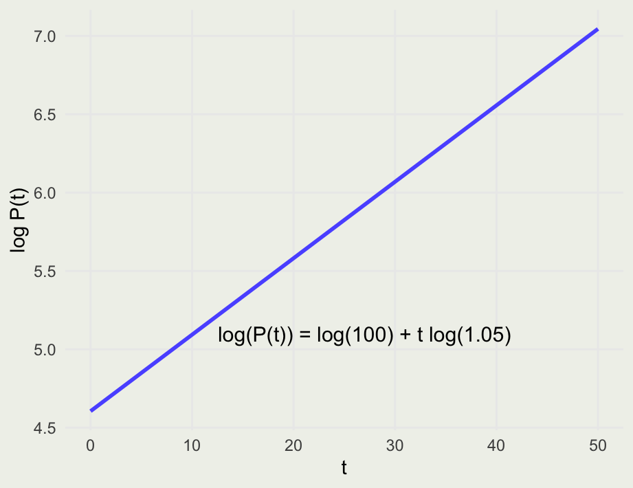
Logs turn growth into a line
\[
\beta \text{ on a log scale}
\quad\Longrightarrow\quad
100\left(e^\beta - 1\right)\% \text{ change}
\]
Softmax can overflow
\[
\operatorname{softmax}(x)_i =
\frac{e^{x_i}}{\sum_{j=1}^N e^{x_j}}
\]
\[
m = \max_j x_j
\]
\[
\operatorname{LSE}(x)
= m + \log\sum_{j=1}^N e^{x_j-m}
\]
\[
\log\operatorname{softmax}(x)_i
= x_i - \operatorname{LSE}(x)
\]
Moon model
downward distance = \(+x\)
\[
m\ddot{x} = mg
\quad\Longrightarrow\quad
\ddot{x} = g
\]
1 kg \(\rightarrow\) mass cancels
\[
x(0) = 0
\qquad
v(0) = 0
\]
\[
v(t) = gt
\]
\[
x(t) = \tfrac{1}{2}gt^2\]
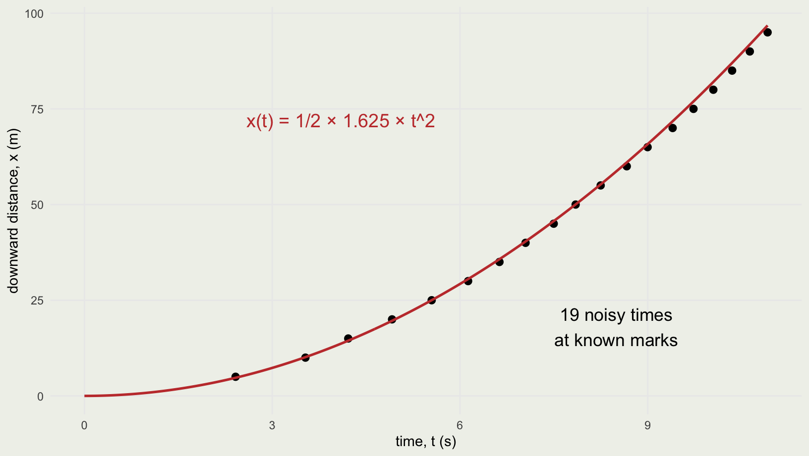
The drop, in data
![]()
reference curve: \(g_{\mathrm{ref}} = 1.625\ \mathrm{m/s^2}\) · not an estimate from these observations
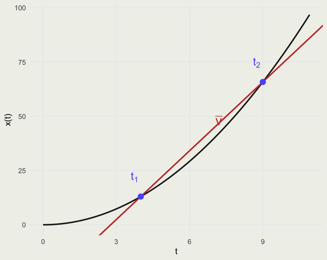
Average velocity is a secant slope
\[
\bar v
= \frac{\Delta x}{\Delta t}
= \frac{x(t_2)-x(t_1)}{t_2-t_1}
\]
\[
\bar v
= \frac{\tfrac12 g(t_2^2-t_1^2)}{t_2-t_1}
= \tfrac12 g(t_1+t_2)
\]
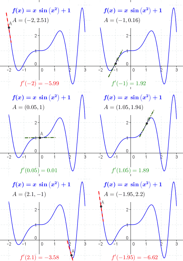
From secant to tangent
\[
\text{secant slope}
= \frac{x(a+h)-x(a)}{h}
\]
\[
v(a)
= \lim_{h\to 0}\frac{x(a+h)-x(a)}{h}
= x'(a)
\]
Position \(\rightarrow\) velocity \(\rightarrow\) acceleration
\[
x(t) = \tfrac12 gt^2
\]
\[
\begin{aligned}
v(t)
&= \lim_{h\to 0}
\frac{\tfrac12 g(t+h)^2-\tfrac12 gt^2}{h} \\
&= \lim_{h\to 0}
\left(gt+\tfrac12 gh\right) \\
&= gt
\end{aligned}
\]
\[
a(t) = v'(t) = x''(t) = g
\]
\[
v(4) \approx 1.62 \times 4 = 6.5\ \mathrm{m/s}\ \text{downward}
\]
Your Turn: another moon
\[
x(t) = 4 + 3t + 5t^2
\]
Find \(x(0)\), \(x(1)\), \(v(0)\), \(v(5)\), \(a(5)\), and \(g\).
\[x(0)=4 \qquad x(1)=12\]
\[v(t)=3+10t\]
\[v(0)=3 \qquad v(5)=53\]
\[a(t)=g=10\]
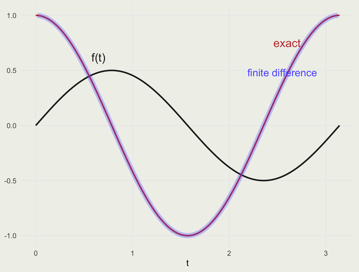
Exact and numerical derivatives
\[
\begin{aligned}
\frac{d}{dt}[\sin t\cos t]
&= \cos t\cos t + \sin t(-\sin t) \\
&= \cos^2t-\sin^2t
\end{aligned}
\]
\[
\frac{\Delta x}{\Delta t}
\approx \frac{dx}{dt}
\]
Your Turn: chain rule
Warm-up:
\[
\frac{d}{dx}\sin(x^2) = 2x\cos(x^2)
\]
Now find
\[
\frac{d}{dx}\left(e^{x^2\cos x}\right).
\]
\[
e^{x^2\cos x}
\left(2x\cos x-x^2\sin x\right)
\]
Mission checkpoint
1 drop \(\longrightarrow\) 19 timed marks
\(g\) to one decimal place?
\(g\) to two decimal places?
oxygen \(\leftrightarrow\) precision
Sessions 6–7
Homework: circular motion
\[
x(t)=R\cos(\omega t),
\qquad
y(t)=R\sin(\omega t),
\qquad
0\le t\le \frac{2\pi}{\omega}
\]
\(R>0\) · \(\omega>0\) · \(T=2\pi/\omega\)
- Write position, velocity, and acceleration functions.
- Plot \(x(t)\) and \(y(t)\) against \(t\); plot \(y\) against \(x\).
- Plot each velocity and acceleration component with its position component.
- Verify
\[
\mathbf a(t) = -\omega^2\mathbf r(t).
\]
- Explain the geometry of \(\mathbf r(t)\), \(\mathbf v(t)\), and \(\mathbf a(t)\).