SMaC: Statistics, Math, and Computing

Applied Statistics for Social Science Research

Eric Novik | Summer 2024 | Session 3

Session 3 Outline

• Transforming data for plotting
• Antiderivative
• Some rules of integration
• Evaluating integrals numerically
• The waiting time distribution

\[ \DeclareMathOperator{\E}{\mathbb{E}} \DeclareMathOperator{\P}{\mathbb{P}} \DeclareMathOperator{\V}{\mathbb{V}} \DeclareMathOperator{\L}{\mathscr{L}} \DeclareMathOperator{\I}{\text{I}} \]

Data transformations

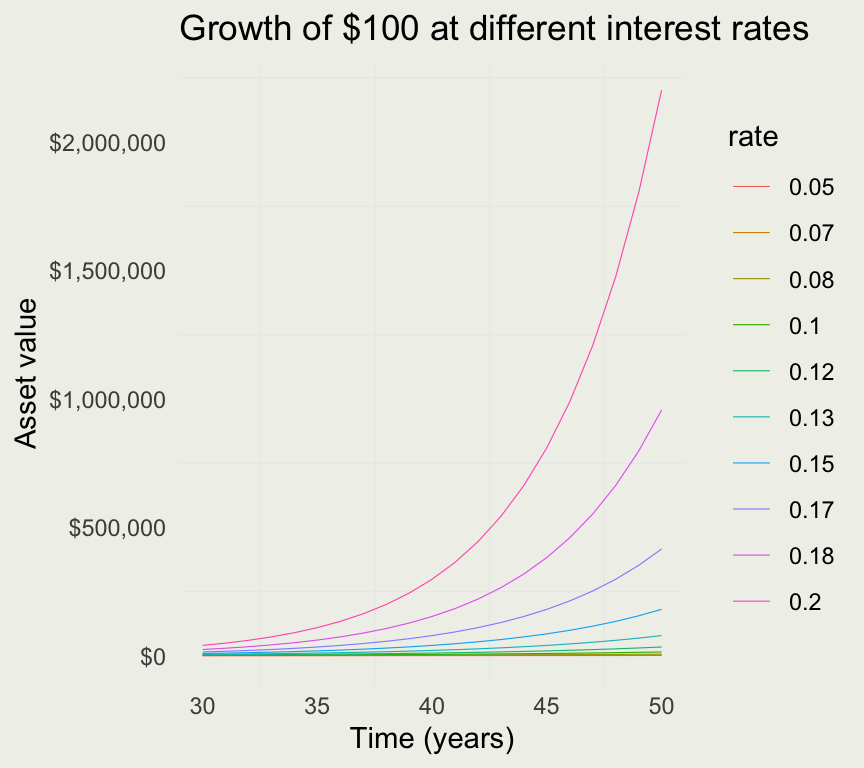
• We saw that continuous compounding does not make such a big difference over time
• How would the value vary by rate?
• We investigate with a common simulate-pivot-plot pattern

Map Function

“The purrr::map* functions transform their input by applying a function to each element of a list or atomic vector and returning an object of the same length as the input.”

• Generate 10 vectors of 100 uniform random realizations, where the first vector has min = 1, second min = 2 … last vector has min = 10, and max = 15 for all
• Now compute the average value of each of the 10 vectors

library(purrr)

x <- 1:10
y <- x |>
  map(\(x) runif(n = 100, min = x, max = 15))

y <- x |>
  map(\(x) runif(n = 100, min = x, max = 15)) |>
  map_dbl(mean)

• Run the code and look inside y after then first function call and after the second. What do you expect to see?

Pivot Functions

“pivot_longer()”lengthens” data, increasing the number of rows and decreasing the number of columns. The inverse transformation is pivot_wider()”

library(tidyr)
head(iris)

  Sepal.Length Sepal.Width Petal.Length Petal.Width Species
1          5.1         3.5          1.4         0.2  setosa
2          4.9         3.0          1.4         0.2  setosa
3          4.7         3.2          1.3         0.2  setosa
4          4.6         3.1          1.5         0.2  setosa
5          5.0         3.6          1.4         0.2  setosa
6          5.4         3.9          1.7         0.4  setosa

iris_long <- iris |> pivot_longer(!Species, names_to = "length_width", values_to = "measure")
head(iris_long)

# A tibble: 6 × 3
  Species length_width measure
  <fct>   <chr>          <dbl>
1 setosa  Sepal.Length     5.1
2 setosa  Sepal.Width      3.5
3 setosa  Petal.Length     1.4
4 setosa  Petal.Width      0.2
5 setosa  Sepal.Length     4.9
6 setosa  Sepal.Width      3  

Data Transformations

• Simulate
• Loops and Maps
• Pivot
• Plot

library(purrr)
library(tidyr)
library(dplyr)
library(ggplot2)

rates <- seq(0.05, 0.20, length = 10)
P <- 100 
time <- seq(1, 50, length = 50)

Pe <- function(A, r, t) A * exp(r * t)
d <- time |>
  map(\(x) Pe(A = P, r = rates, t = x)) 
class(d)

[1] "list"

d[[1]][1:4]

[1] 105.1271 106.8939 108.6904 110.5171

names(d) <- as.character(time)
d <- as_tibble(d)

1	2	3
105.1271	110.5171	116.1834
106.8939	114.2631	122.1403
108.6904	118.1360	128.4025
110.5171	122.1403	134.9859
112.3745	126.2802	141.9068
114.2631	130.5605	149.1825
116.1834	134.9859	156.8312
118.1360	139.5612	164.8721
120.1215	144.2917	173.3253
122.1403	149.1825	182.2119

• Modern R usage offers a lot of shortcuts but those may be confusing to beginners.
• In particular, R loops have mostly been replaced with map() functions.
• We recommend purrr::map() functions instead of R’s *apply().

rates <- seq(0.05, 0.20, length = 10)
P <- 100 
time <- seq(1, 5, length = 50)

Pe <- function(A, r, t) A * exp(r * t)
time |> map(\(x) Pe(A = P, r = rates, t = x)) 

# above is a shortcut for
map(time, function(x) Pe(A = P, r = rates, t = x))

# and the above is a shortcut for the following loop
l <- list()
for (i in seq_along(time)) {
  l[[i]] <- Pe(A = P, r = rates, t = time[i])
}

library(tidyr)
# add rates as a column
d <- d %>% mutate(rate = 
            round(rates, 2) |>
              as.character())

# convert from wide format to long
d <- d %>% 
  pivot_longer(!rate, 
               names_to = "year", 
               values_to = "value") 

d$year <- as.numeric(d$year)

Here is a cheat sheet explaining tidyr functions.

rate	year	value
0.05	1	105.1271
0.05	2	110.5171
0.05	3	116.1834
0.05	4	122.1403
0.05	5	128.4025
0.05	6	134.9859
0.05	7	141.9068
0.05	8	149.1825
0.05	9	156.8312
0.05	10	164.8721

p <- ggplot(d, aes(year, value))
p + geom_line(aes(color = rate), linewidth = 0.2) +
  scale_y_continuous(labels = 
          scales::dollar_format()) +
  xlab("Time (years)") + 
  ylab("Asset value") +
  ggtitle("Growth of $100 at different interest rates")

d |> group_by(rate) |> 
  summarise(y50 = last(value)) |>
  knitr::kable()

rate	y50
0.05	1218.249
0.07	2803.162
0.08	6450.009
0.1	14841.316
0.12	34149.510
0.13	78577.199
0.15	180804.241
0.17	416026.201
0.18	957266.257
0.2	2202646.579

Your Turn

• Data
• Instructions
• Output

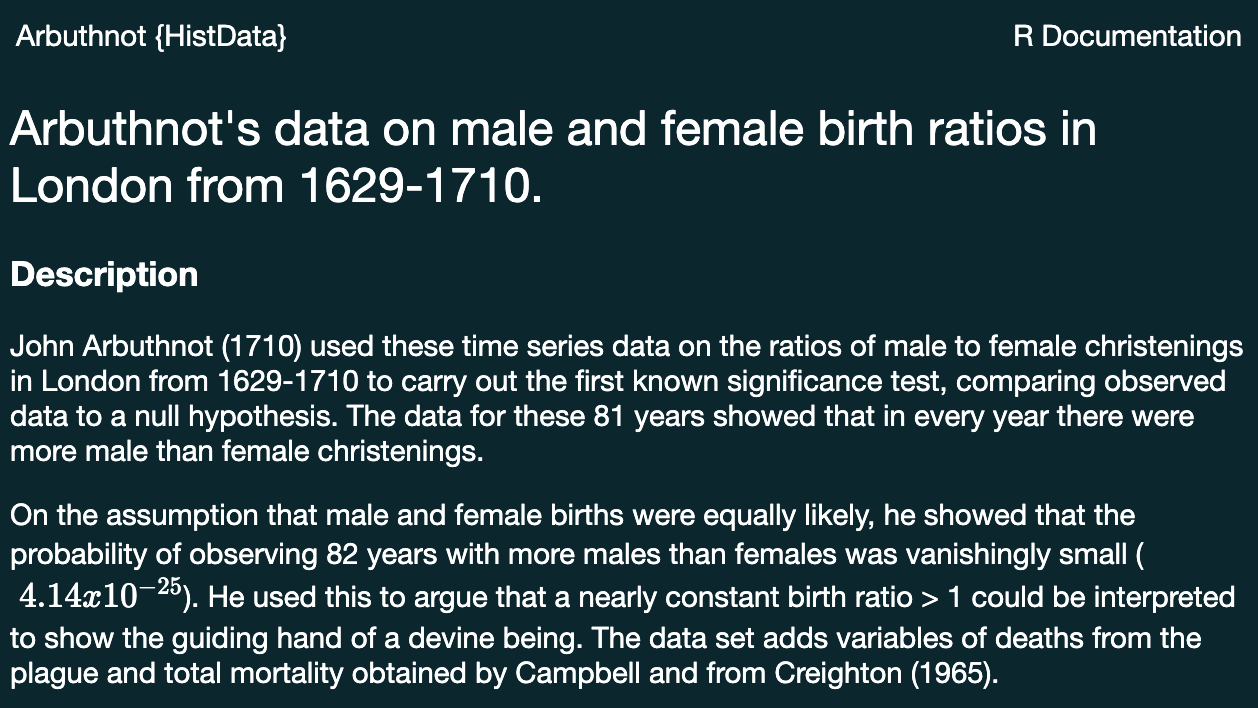
• Run the following command: install.packages('HistData')
• Followed by library(HistData)
• Tale a look at the Arbuthnot dataset: ?Arbuthnot

Year	Males	Females	Plague	Mortality	Ratio	Total
1629	5218	4683	0	8771	1.114243	9.901
1630	4858	4457	1317	10554	1.089971	9.315
1631	4422	4102	274	8562	1.078011	8.524
1632	4994	4590	8	9535	1.088017	9.584
1633	5158	4839	0	8393	1.065923	9.997
1634	5035	4820	1	10400	1.044606	9.855

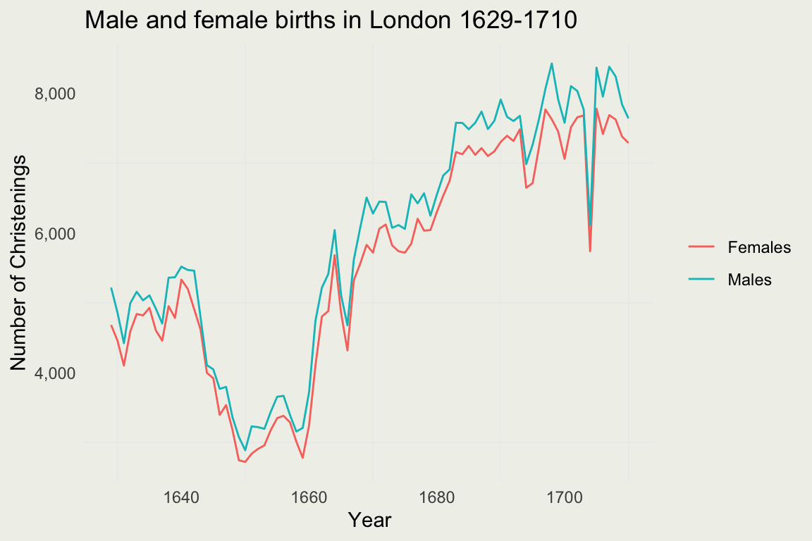
• Use the tools to produce the plot the looks something like this.
• Bonus: compute the ratio of female births and plot it.

Integral Calculus

• Integration plays a central role in Statistics
• It is a way to compute Expectations and Event Probabilities
• In Bayesian Statistics, we use integration to compute posterior distributions of the unknowns
• In Frequentist Statistics, we use derivatives to find the most likely values of the unknowns

• Unknowns are sometimes called parameters, like our \(a\) and \(b\), in the \(x(t) = a + bt^2\) model

Intuition Behind Integration

• Integration is a continous analog of summation
• You can also think of an integral as undoing a derivative
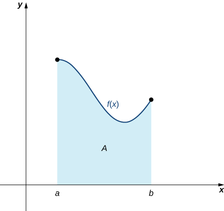
• You can also think of it as a signed area under a function \(f\)
• In modern applications, integration is almost always done numerically on the computer
• But it helps to understand what what the computer is doing

From Velocity to Postion Functions

• Antiderivative
• Plot

• Recal our position function \(x(t) = 2 + 3t^2\)
• We found the velocity function by differentiating and we can almost get back the position function by integrating.

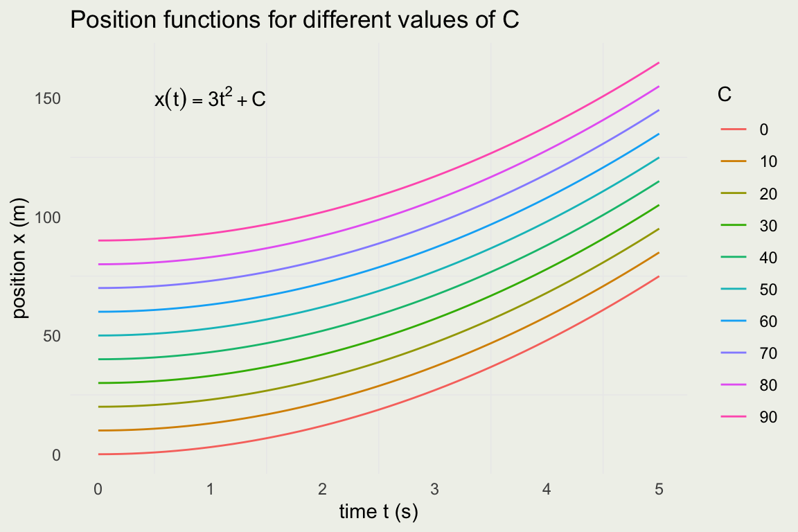
\[ \begin{eqnarray} v(t) & = & \frac{d}{dt} \left( 2 + 3t^2 \right) = 6t \\ x(t) & = & \int{6t\, dt} = 3t^2 + C \end{eqnarray} \]

• Why almost? Look at the constant \(2\) in \(\frac{d}{dt}(2 + 3t^2)\). You can replace it with any other constant and the result will still be \(6t\).

• To put it another way, to characterize the position fucntion you need to know the intial position and you can’t get that from the velocity function alone.

The position function for different values of initial position \(C\). Notice that the only thing that changes is the intercept.

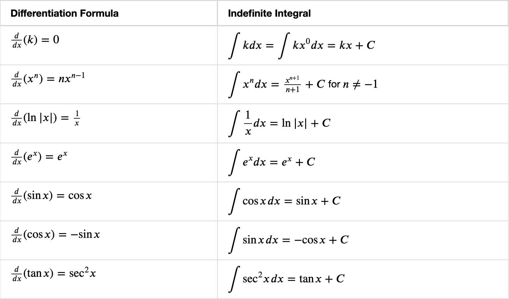
Some Common Integrals

Techniques of Intergration

• Integral, like a derivative, is a linear operator:

\[ \begin{eqnarray} \int [f(x) + g(x)] \, dx &=& \int f(x) \, dx + \int g(x) \, dx \\ \int [c \cdot f(x)] \, dx &=& c \int f(x) \, dx \end{eqnarray} \]

• Unlike derivatives, there are generablly no rules for finding integrals

• Most integrals do not have a closed-form, analytical solutions. This is true for almost all integrals in statistics.

• In one or two dimentions, it is easy to evaluate most integrals numerically.

• In higher dimentions, you need very sophisticated methods that rely on Markov Chain Monte Carlo (MCMC). We will not cover MCMC in this course.

• For simple integrals we can somtimes find a closed-form solution by relying on u-substitution and integration by parts.

Playing with Integrals

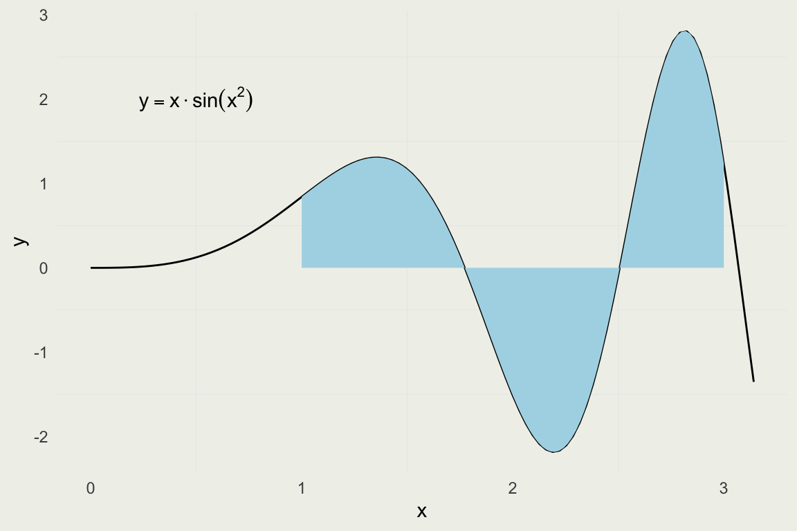
• Given our intuition for integrals being singed areas, let’s see how to compute them analytically and numerically.
• Warning: these techniques only work in low dimentions. For high dimentional integrals you need to use MCMC.
• Suppose we want evaluate the integral \(\int_{1}^{3} x \sin(x^2)\, dx\)

Constructing a Riemann Sum

riemann <- function(f, lower, upper, step_size) {
  step <- seq(lower, upper, by = step_size)
  s <- 0 # initialize the sum
  for (i in 2:length(step)) {
    # multiply base by the height of the rectangle
    area <- step_size * f(step[i]) 
    s <- s + area
  }
  return(s)
}

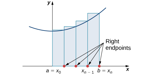
Notice that the function takes a function as an argument. These are called higher order functions.

Evaluating the Integral

f <- function(x) x * sin(x^2)
x <- seq(0, pi, len = 100)

riemann(f, 1, 3, 0.01)

[1] 0.7275414

# compute using R's integrate function
integrate(f, 1, 3)

0.7257163 with absolute error < 1.3e-09

Integrating Analytically

• Most integrals can’t be evaluated analytically but we can do \(\int x \sin(x^2)\, dx\).
• We make a substitution. Let \(u = x^2\), then \(du/dx = 2x\) and \(dx = \frac{1}{2 \sqrt{u}}du\)

\[ \begin{eqnarray} \int \sqrt{u} \cdot \sin(u) \frac{1}{2\sqrt{u}}du & = & \\ \frac{1}{2}\int \sin(u)\, du & = & \\ -\frac{1}{2} \cos(u) & = & -\frac{1}{2} \cos(x^2) \end{eqnarray} \]

Comparing the Results

• Using R’s integrate function:

integrate(f, 1, 3)

0.7257163 with absolute error < 1.3e-09

• Using the analytical solution

f1 <- function(x) -1/2 * cos(x^2)

f1(3) - f1(1)

[1] 0.7257163

• The universe is in balance!

Analytical Integration on the Computer

• When in doubt, you can always try WolframAlpha

• Python library SymPy through R pacakge caracas

library(caracas); library(stringr)
add_align <- function(latex) {
  str_c("\\begin{align} ", latex, " \\end{align}")
}
add_int <- function(latex) {
  str_c("\\int ", latex, "\\, dx")
}
x <- symbol('x'); f <- x^2 / sqrt(x^2 + 4)
tex(f) %>% add_int() %>% str_c(" =") %>% add_align() %>% cat()

\[\begin{align} \int \frac{x^{2}}{\sqrt{x^{2} + 4}}\, dx = \end{align}\]

int(f, x) %>% tex() %>% add_align() %>% cat()

\[\begin{align} \frac{x \sqrt{x^{2} + 4}}{2} - 2 \operatorname{asinh}{\left(\frac{x}{2} \right)} \end{align}\]

Your Turn: Waiting Time

• There is s famous distribution in statistics called Exponential distribution
• Its probability density function (PDF) is given by:

\[ f(x) = \lambda e^{-\lambda x}, \, x > 0, \text{and } \lambda > 0 \]

• This distribution is sometimes called the waiting time (to some event) distribution, where \(\lambda\) is the rate of events we expect

• One property of this distribution is that no matter how long you wait, the probability of seeing an event remains the same.

• One of the properties of the PDF is that it must integrate to 1

• Let’s check that it’s true

\[ \int_{0}^{\infty} \lambda e^{-\lambda x} dx = \]

Ingegration by Parts

\[ \begin{eqnarray} (f g)' & = & f'g + g'f \\ \int (f g)' \, dx & = & \int f'g dx + \int g'f \, dx \\ fg & = & \int f'g \, dx + \int g'f \, dx \\ \int f g' \, dx & = & fg - \int f' g \, dx \\ u & = & f(x) \\ v & = & g(x) \\ du & = & f'(x) \, dx \\ dv & = & g'(x) \, dx \\ \int u \, dv & = & uv - \int v \, du \end{eqnarray} \]

Exponential Growth (again)

Recall, at the beginning we defined an exponential growth with the following differential equation:

\[ \frac{dy(t)}{dt} = k \cdot y(t) \]

We can now solve it:

\[ \begin{align*} \frac{1}{y} \, dy &= k \, dt \\ \int \frac{1}{y} \, dy &= \int k \, dt \\ \log(y) &= k \cdot t + C \\ y(t) &= y_0 \cdot e^{kt} \end{align*} \]

Homework

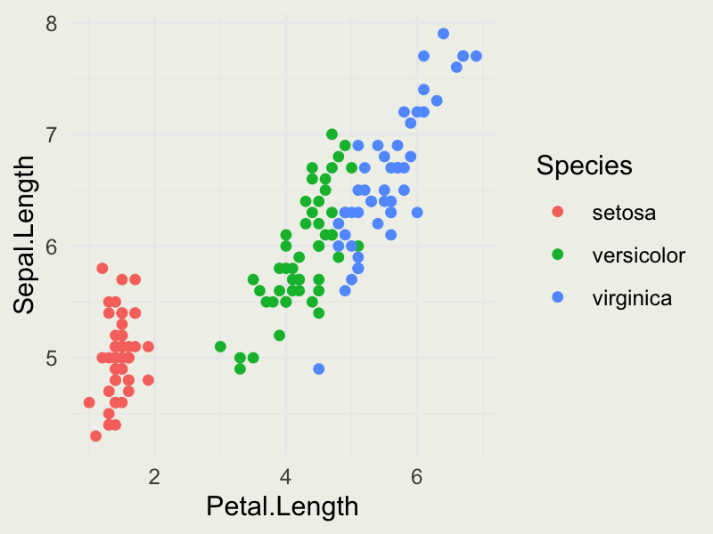
• Take a look at dataset iris (?iris)
• Compute the overall average Sepal.Length, Sepal.Width, Petal.Length, Petal.Width
• Compute the average by each Species of flower (hint: use group_by and summarise functions from dplyr)
• Produce the plot that looks like this:

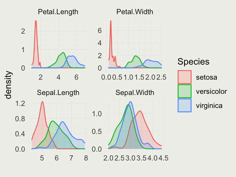
• Produce the plot that looks like this: (check out geom_density and facet_wrap functions)

• Compute the following integral and show the steps:

\[ \int 2x \cos(x^2)\, dx \]

• Evaluate this integral (on paper) from \(0\) to \(2\pi\) and use R’s integrate function to validate your answer.