SMaC: Statistics, Math, and Computing

Applied Statistics for Social Science Research

Eric Novik | Summer 2024 | Session 4

Session 4 Outline

• What is probability?
• How does it relate to statistics?
• Sample spaces and arithmetic of sets
• How to count without counting
• Conditional probability
• Independence and Bayes rule
• Examples
  • COVID testing
  • Birthday problem
  • Leibniz’s error
  • Monte Hall

What is Probability

• Statistics is the art of quantifying uncertainty, and probability is the language of statistics
• Probability is a mathematical object
• People argue over the interpretation of probability
• People don’t argue about the mathematical definition of probability

Andrei Kolmogorov (1903 — 1987)

\[ \DeclareMathOperator{\E}{\mathbb{E}} \DeclareMathOperator{\P}{\mathbb{P}} \DeclareMathOperator{\V}{\mathbb{V}} \DeclareMathOperator{\L}{\mathscr{L}} \DeclareMathOperator{\I}{\text{I}} \]

Laplace’s Demon

We may regard the present state of the universe as the effect of its past and the cause of its future. An intellect which at any given moment knew all of the forces that animate nature and the mutual positions of the beings that compose it, if this intellect were vast enough to submit the data to analysis, could condense into a single formula the movement of the greatest bodies of the universe and that of the lightest atom; for such an intellect nothing could be uncertain, and the future just like the past would be present before its eyes.

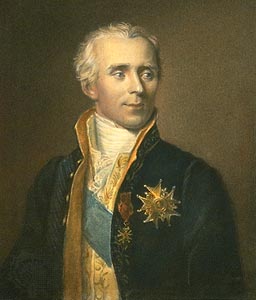
Marquis Pierre Simon de Laplace (1729 — 1827)

“Uncertainty is a function of our ignorance, not a property of the world”

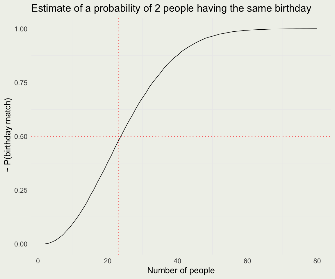
Sample Spaces

• A sample space which we will call \(S\) is a set of all possible outcomes \(s\) of an experiment.

• If we flip a coin twice, our sample space has \(4\) elements: \(\{TT, TH, HT, HH\}\).

• An event \(A\) is a subset of a sample space. We say that \(A \subseteq S\)

• Possible events: 1) At least one \(T\); 2) The first one is \(H\); 3) Both are \(T\); 4) Both are neither \(H\) nor \(T\); etc

Sample Spaces and De Morgan

• A compliment of an event \(A\) is \(A^c\). Formally, this is \(A^c = \{s \in S: s \notin A\}\)

• Suppose, \(S = \{1, 2, 3, 4\}\), \(A = \{1, 2\}\), \(B = \{2, 3\}\), and \(C = \{3, 4\}\)

• Then, the union of A and B is \(A \cup B = \{1, 2, 3\}\), \(A \cap B = \{2\}\), \(A^c = \{3, 4\}\), and \(B^c = \{1, 4\}\). And \(A \cap C = \{\emptyset \}\)

• De Morgan (1806 — 1871) said that:

  • \((A \cup B)^c = A^c \cap B^c\) and
  • \((A \cap B)^c = A^c \cup B^c\)

• In our case, \((A \cup B)^c = (\{1, 2, 3\})^c = \{4\} = (\{3, 4\} \cap \{1, 4\})\)

• Your Turn: Compute \((A \cap B)^c = A^c \cup B^c\)

Naive Definition

• Naive definition of probability is an assumption that every outcome is equally likely
• In that case, \(\P(A) = \frac{\text{number of times A occurs}}{\text{number of total outcomes}}\)
• What is the probability of rolling an even number on a six-sided die?
  • \(\P(\text{Even Number}) = \frac{3}{6} = \frac{1}{2}\)
• What is the probability of rolling a prime number?
  • \(\P(\text{Prime Number}) =\)

Counting

• Your mom feels probabilistic, so she asks you to flip a coin. If it lands heads, you get pizza for dinner, and if lands tails, you get broccoli. You flip again for dessert. If it lands heads, you get ice cream, and if it lands tails, you get a cricket cookie. Assume you are not a fan of veggies and insects. What is the probability of having a completely disappointing meal? What is the probability of being partly disappointed?

• From Blitzstein and Chen (2015): Suppose that 10 people are running a race. Assume that ties are not possible and that all 10 will complete the race, so there will be well-defined first place, second place, and third place winners. How many possibilities are there for the first, second, and third place winners?

Basic Counting

• How many permutations of \(n\) object are there?
• Sampling with replacement (order matters): you select one object from \(n\) total objects, \(k\) times (and put it back each time).
• Sampling without replacement (order matters): same as above, but you don’t put them back

Binomial coefficient

• How many ways are there to choose a number of subsets from a set; e.g., how many two-person teams can be formed from five people? (here, John and Jane is the same set as Jane and John)

\[ {n \choose k} = \frac{n!}{(n - k)! k!} = {n \choose n-k} \]

• What is the probability of the full house in poker? (3 cards of the same rank and 2 cards of the other rank)
• How many unique shuffles are there in one deck of 52 cards?

Birthday Problem

• Problem Description
• Simulation
• Plot

There are \(j\) people in a room. Assume each person’s birthday is equally likely to be any of the 365 days of the year (excluding February 29) and that people’s birthdays are independent. What is the probability that at least one pair of group members has the same birthday?

n <- 1e5
n_people <- 80 
j <- 2:n_people
days <- 1:365 

find_match <- function(x, d) {
  y <- sample(d, x, replace = TRUE)
  match_found <- length(unique(y)) < length(y)
}

prop <- numeric(n_people - 1)
for (i in seq_along(j)) {
  matches <- replicate(n, find_match(i, days))
  prop[i] <- mean(matches)
}

Birthday Analysis

• Let’s say we have \(j\) people. There are 365 ways in which the first person can get a birthday, 365 for the second, and so on, assuming no twins. So the denominator is \(365^j\)

• For the numerator, it is easier to compute a probability of no match. Let’s say we have three people in the room. The numerator would be \(365 \cdot 364 \cdot 363\), the last term being \(365 - j + 1\)

\[ \P(\text{At least one match}) = 1 - P(\text{No match}) = \\ 1 - \frac{\prod_{i = 0}^{j-1} (365-i)}{365^j} = 1 - \frac{365 \cdot 364 \cdot 363 \cdot \,... \, \cdot (365 - j + 1)}{365^j} \]

• (Number of People, Probability of a match):

(2, 0); (3, 0.01); (4, 0.02); (5, 0.03); (6, 0.04); (7, 0.06); (8, 0.07); (9, 0.09); (10, 0.12); (11, 0.14); (12, 0.17); (13, 0.19); (14, 0.22); (15, 0.25); (16, 0.28); (17, 0.32); (18, 0.35); (19, 0.38); (20, 0.41); (21, 0.44); (22, 0.48); (23, 0.51)

Probability

• Probability \(\P\) assigns a real number to each event \(A\) and satisfies the following axioms:

\[ \begin{eqnarray} \P(A) & \geq & 0 \text{ for all } A \\ \P(S) & = & 1 \\ \text{If } \bigcap_{i=1}^{\infty}A_i = \{\emptyset \} & \implies & \P\left( \bigcup_{i=1}^{\infty}A_i \right) = \sum_{i=1}^{\infty}\P(A_i) \end{eqnarray} \]

• For \(S = \{1, 2, 3, 4\}\), where \(s_i = 1/4\), and \(A = \{A_1, A_2\}\), where \(A_1 = \{1\}\) and \(A_2 = \{2\}\). Verify that all 3 axioms hold.

Some Consequences

\[ \begin{eqnarray} \P\{\emptyset\} & = & 0 \\ A \subseteq B & \implies & \P(A) \leq \P(B) \\ \P(A^c) & = & 1 - P(A) \\ A \cap B = {\emptyset} & \implies & \P(A \cup B) = \P(A) + \P(B) \\ \P(A \cup B) & = & \P(A) + \P(B) - \P(A \cap B) \end{eqnarray} \newcommand{\indep}{\perp \!\!\! \perp} \]

• The last one is called inclusion-exclusion
• Two events are independent \(A \indep B\) if:

\[ \P(A \cap B) = \P(A) \P(B) \]

Some Examples

• Simulation
• Analysis
• Your Turn

You flip a fair coin four times. What is the probability that you get one or more heads?

one_or_more <- function() {
  flips <- sample(c(1, 0), size = 4, replace = TRUE)
  if (mean(flips) >= 1/4) {
    return(TRUE)
  } else {
    return(FALSE)
  }
}
# flip the coin 10,000 times
x <- replicate(1e4, one_or_more())
mean(x)

[1] 0.9366

Let \(A\) be the probability of at least one Head. Then \(A^c\) is the probability of all Tails. Let \(B_i\) be the event of Tails on the \(i\)th trial.

\[ \begin{eqnarray} \P(A) = 1 - \P(A^c) & = & \\ 1 - \P(B_1 \cap B_2 \cap B_3 \cap B_4) & = & \\ 1 - \P(B_1)\P(B_2)\P(B_3)\P(B_4) & = & \\ 1 - \left( \frac{1}{2} \right)^4 = 1 - \frac{1}{16} = 0.9375 \end{eqnarray} \]

• Modify the function so that instead of 1 or more from 4 trials, it computes 1 or more from \(n\) trials.

• Modify it so it computes \(x\) or more from \(n\) trials and simulate at least 2 Heads out of 5 trials.

• Can you solve it analytically to validate your simulation results?

Conditional Probability

Conditioning is the soul of statistics — Joe Blitzstein

• Think of conditioning as the probability in reduced sample spaces since when we condition, we are looking at the subset of \(S\) where some events already occurred.

• Note: In some texts, \(AB\) is used as a shortcut for \(A \cap B\). You can’t multiply events, but you can multiply their probabilities.

\[ \P(A | B) = \frac{\P(A \cap B)}{\P(B)} \]

• Note that \(\P(A|B)\) and \(\P(B|A)\) are different things. Doctors and lawyers confuse those all the time.

• Two events are independent iff \(\P(A | B) = \P(A)\). In other words, learning \(B\) does not improve our estimate of \(\P(A)\).

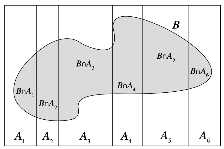
Law of Total Probability and Bayes

• LOTP
• Bayes

\[ \P(B) = \sum_{i=1}^{n} \P(B | A_i) \P(A_i) \]

• We take the definition of conditional probability and expand the numerator and denominator:

\[ \P(A|B) = \frac{\P(B \cap A)}{\P(B)} = \frac{\P(B|A) \P(A)}{\sum_{i=1}^{n} \P(B | A_i) \P(A_i)} \]

• We call \(\P(A)\), prior probability of \(A\) and \(\P(A|B)\) a posterior probability of \(A\) after we learned \(B\).

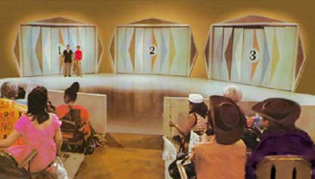
Example: Medical Testing

• Derivation
• Discussion

The authors calculated the sensitivity and specificity of the Abbott PanBio SARS-CoV-2 rapid antigen test to be 45.4% and 99.8%, respectively. Suppose the prevalence is 0.1%.

• Your child tests positive on this test. What is the probability that she has COVID? That is, we want to know \(P(D^+ | T^+)\)
• \(\text{Specificity } := P(T^- | D^-) = 0.998\)
• False positive rate \(\text{FP} := 1 - \text{Specificity } = 1 - P(T^- | D^-) = P(T^+ | D^-) = 0.002\)
• \(\text{Sensitivity } := P(T^+ | D^+) = 0.454\)
• False negative rate \(\text{FP} := 1 - \text{Sensitivity } = 1 - P(T^+ | D^+) = P(T^- | D^+) = 0.546\)
• Prevalence: \(P(D^+) = 0.001\)

\[ \begin{eqnarray} P(D^+ | T^+) = \frac{P(T^+ | D^+) P(D^+)}{P(T^+)} & = & \\ \frac{P(T^+ | D^+) P(D^+)}{\sum_{i=1}^{n}P(T^+ | D^i) P(D^i) } & = & \\ \frac{P(T^+ | D^+) P(D^+)}{P(T^+ | D^+) P(D^+) + P(T^+ | D^-) P(D^-)} & = & \\ \frac{0.454 \cdot 0.001}{0.454 \cdot 0.001 + 0.002 \cdot 0.999} & \approx & 0.18 \end{eqnarray} \]

• The answer, 18%, is very sensitive to the prevalence of disease, or in our language, to the prior probability of an infection
• At the time of the test, the actual prevalence was estimated at 4.8%, not 0.1%, which would change our answer by a lot: \(\P(D^+ | T^+) \approx 0.92\)
• Lesson: don’t rely on intuition and check the prior

Example: Leibniz’s Error

• You have two 6-sided fair dice. You roll the dice and compute the sum. Which one is more likely 11 or 12?

Example: Monte Hall