SMaC: Statistics, Math, and Computing

Applied Statistics for Social Science Research

Eric Novik | Summer 2024 | Session 5

Session 5 Outline

  • Random variables
  • Bernoulli, Binomial, Geometric
  • PDF and CDF
  • LOTUS
  • Poisson
  • Expectations, Variance
  • St. Petersburg Paradox
  • Normal

\[ \DeclareMathOperator{\E}{\mathbb{E}} \DeclareMathOperator{\P}{\mathbb{P}} \DeclareMathOperator{\V}{\mathbb{V}} \DeclareMathOperator{\L}{\mathscr{L}} \DeclareMathOperator{\I}{\text{I}} \]

Random Variables are Not Random

  • It would be inconvenient to enumerate all possible events to describe a stochastic system

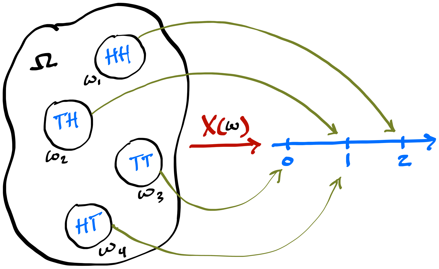
  • A more general approach is to introduce a function that maps sample space \(S\) onto the Real line

  • For each possible outcome \(s\), random variable \(X(s)\) performs this mapping

  • This mapping is deterministic. The randomness comes from the experiment, not from the random variable (RV)

  • While it makes sense to talk about \(\P(A)\), where \(A\) is an event, it does not make sense to talk about \(\P(X)\), but you can say \(\P(X(s) = x)\), which we usually write as \(\P(X = x)\)

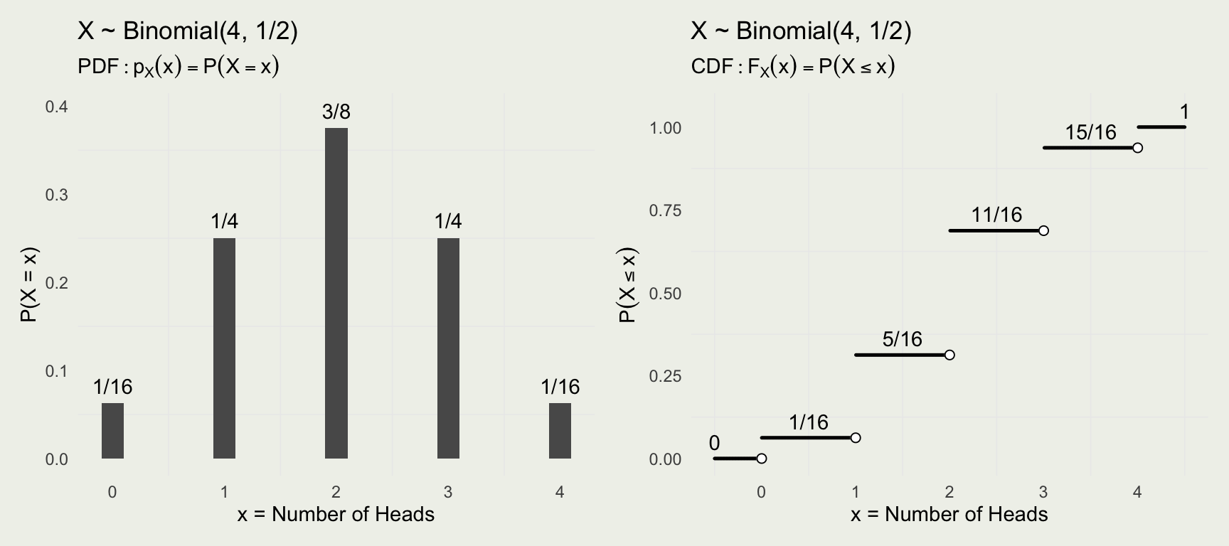
  • Let \(X\) be the number of Heads in two coin flips. You flip the coin twice, and you get \(HH\). In this case, \(s = {HH}\), \(X(s) = 2\), while \(S = \{TT, TH, HT, HH\}\)

  • Random variable \(X\) for the number of Heads in two flips

Characterising Random Variables

  • Two ways of describing an RV are CDF (Cumulative Distribution Function) and PMF (Probability Mass Function) for discrete RVs and PDF (Probability Density Function) for continuous RVs. There are other ways, but we will stick with CDF and P[D/M]F.
  • CDF \(F_X(x)\) is a function of \(x\) and is bounded between 0 and 1:

\[ F_X(x) = \P(X \leq x) \]

  • PMF (for discrete RVs only) \(f_X(x)\) is a function of \(x\)

\[ f_X(x) = \P(X = x) \]

  • You can get from \(f_X\) to \(F_X\) by summing. Let’s say \(x = 4\). In that case:

\[ F_X(4) = \P(X \leq 4) = \sum_{i = 4,3,2,...}\P(X = i) \]

  • In R, PMFs and PDFs start with the letter d. For example dbinom() and dnormal() refer to binomial PMF and normal PDF

  • CDFs start with p, so pbinom() and pnorm()

  • Inverse CDFs or quantile functions, start with q so qbinom() and so on

  • Random number generators start with r, so rbinom()

  • A binomial RV, which we will define later, represents the number of successes in N trials. In R, the PMF is dbinom() and CDF is pbinom()

  • Here is the full function signature: dbinom(x, size, prob, log = FALSE)

    • x is the number of successes, size is the number of trials N, prob is the probability of success in each trial \(\theta\), and log is a flag asking if we want the results on the log scale.

Binomial RV

  • Bernoulli RV is one coin flip with a set probability of success (say Heads)

  • If \(X \sim \text{Bernoulli}(\theta)\), the PMF can be written directly as \(\P(X = x) = \theta^x (1 - \theta)^{1-x}, \, x \in \{0, 1\}\)

  • Binomial can be thought of as the sum of \(N\) independent Bernoulli trials. We can also write:

\[ \text{Bernoulli}(x~|~\theta) = \left\{ \begin{array}{ll} \theta & \text{if } x = 1, \text{ and} \\ 1 - \theta & \text{if } x = 0 \end{array} \right. \]

  • We can write the Binomial PMF, \(X \sim \text{Binomial}(N, \theta)\) this way:

\[ \text{Binomial}(x~|~N,\theta) = \binom{N}{x} \theta^x (1 - \theta)^{N - x} \]

\(\text{Binomial}(x~|~N=4,\theta = 1/2)\)

library(patchwork)
library(MASS)

N <- 4 # Number of successes out of x trials

# compute and plot the PMF
pmf <- dbinom(x = 0:N, size = N, prob = 1/2)
d <- data.frame(x =  0:N, y = pmf)
p1 <- ggplot(d, aes(x, pmf))
p1 <- p1 + geom_col(width = .2) + 
  geom_text(aes(label = fractions(pmf)), nudge_y = 0.02) +
  ylab("P(X = x)") + xlab("x = Number of Heads") +
  ggtitle("X ~ Binomial(4, 1/2)",
          subtitle = expression(PDF: p[X](x) == P(X == x)))

# compute and plot the CDF
x <- seq(-0.5, 4.5, length = 500)
cdf <- pbinom(q = x, size = N, prob = 1/2)
d <- data.frame(q = x, y = cdf)
dd <- data.frame(x = seq(-0.5, 4.5, by = 1), cdf = unique(cdf), x_empty = 0:5)
p2 <- ggplot(d, aes(x, cdf)) 
p2 <- p2 + geom_point(size = 0.2) + 
  geom_text(aes(x, cdf, label = fractions(cdf)), data = dd, nudge_y = 0.05) +
  geom_point(aes(x_empty, cdf), data = dd[-6, ], size = 2, color = 'white') +
  geom_point(aes(x_empty, cdf), data = dd[-6, ], size = 2, shape = 1) +
  ggtitle("X ~ Binomial(4, 1/2)",
          subtitle = expression(CDF: F[X](x) == P(X <= x))) +
  ylab(expression(P(X <= x))) + xlab("x = Number of Heads")

p1 + p2

Binomial in R

# What is the probability of getting 2 Heads out of 5 fair trials?
N <- 5; x <- 2
dbinom(x = x, size = N, prob = 0.5) |> fractions()
[1] 5/16
# What is the binomial PMF: P(X = x), for N = 5, p = 0.5?
N <- 5; x <- -2:7 # notice we range x over any integers
dbinom(x = x, size = N, prob = 0.5) |> fractions()
 [1]    0    0 1/32 5/32 5/16 5/16 5/32 1/32    0    0
# Verify that the PMF sums to 1
sum(dbinom(x = x, size = N, prob = 0.5))
[1] 1
# What is the probability of 3 heads or fewer
pbinom(3, size = N, prob = 0.5) |> fractions()
[1] 13/16
# compute the CDF: P(X <= x), for N = 5, p = 0.5
pbinom(x, size = N, prob = 0.5) |> fractions()
 [1]     0     0  1/32  3/16   1/2 13/16 31/32     1     1     1
# get from the PMF to CDF; cumsum() is the cumulative sum function
dbinom(x = x, size = N, prob = 0.5) |> cumsum() |> fractions()
 [1]     0     0  1/32  3/16   1/2 13/16 31/32     1     1     1
  • Your Turn: Suppose the probability of success is 1/3, N = 10. What is the probability of 6 or more successes? Compute it with a PMF first and verify with the CDF.

Geometric RV

  • Geometric is a discrete waiting time distribution, and Exponential is its continuous analog
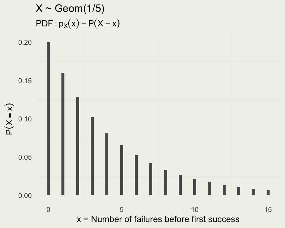
  • If \(X\) is the number of failures before first success \(X \sim \text{Geometric}(\theta)\), where \(\theta\) is probability of success
  • Example: We keep flipping a coin until we get success, say Heads
    • Say we flip five times, which means we get the following sequence: T T T T H
    • The probability of this sequence is: \((\frac{1}{2})^4 (\frac{1}{2})^1\)
    • Notice this is the only way to get this sequence
  • If \(x\) is the number of failures, the PMF is \(P(X = x) = (1 - \theta)^x \theta\), where \(x = 0, 1, 2, ...\)
  • To check if this is a valid PMF, we need to sum over all \(x\):

\[ \begin{align} \sum_{x = 0}^{\infty} \theta (1 - \theta)^x = \theta \sum_{x = 0}^{\infty} (1 - \theta)^x \\ \text{Let } u = 1 - \theta \\ \theta \sum_{x = 0}^{\infty} u^x = \theta \frac{1}{1-u} = \theta \frac{1}{1-1 + \theta} = \frac{\theta}{\theta} = 1 \end{align} \]

  • The last bit comes from geometric series for \(|u| < 1\)
  • The probability of T T T H (x = 3 failures) when \(\theta = 1/2\), has to be \((1/2)^4\) or \(1/16\)
x <- 3; theta <- 1/2
dgeom(x = x, prob = theta) |> fractions()
[1] 1/16
  • If \(\theta = 1/3\), the probability of the same sequence has to be \((2/3)^3 \cdot 1/3 = 8/81\)
x <- 3; theta <- 1/3
dgeom(x = x, prob = theta) |> fractions()
[1] 8/81
  • The PMF is unbounded, but it converges to 1 as demonstrated before
x <-  0:15
theta <- 1/5
y <- dgeom(x = x, prob = theta)
d <- data.frame(x, y)
p <- ggplot(d, aes(x, y))
p + geom_col(width = 0.2) +
xlab("x = Number of failures before first success") +
 ylab(expression(P(X == x))) +
ggtitle("X ~ Geom(1/5)", 
 subtitle = expression(PDF: p[X](x) == P(X == x)))

Let’s consider the infinite geometric series:

\[ S = \sum_{x=0}^{\infty} u^x = u^0 + u^1 + u^2 + u^3 + \dots \] This can be written explicitly as: \[ S = 1 + u + u^2 + u^3 + \dots \]

Next, multiply the entire series by \(u\):

\[ uS = u \cdot (1 + u + u^2 + u^3 + \dots) \]

This results in: \[ uS = u + u^2 + u^3 + u^4 + \dots \]

Now, subtract the equation for \(uS\) from the equation for \(S\):

\[ S - uS = (1 + u + u^2 + u^3 + \dots) - (u + u^2 + u^3 + u^4 + \dots) \]

Notice that all terms on the right-hand side except the first term (which is 1) cancel out:

\[ S - uS = 1 \]

Factor the left-hand side:

\[ S(1 - u) = 1 \]

Finally, solve for \(S\):

\[ S = \frac{1}{1 - u} \]
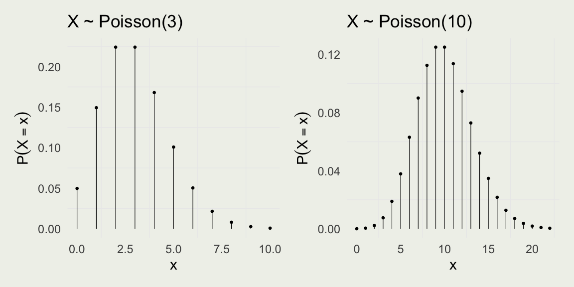
Expectations

  • An expectation is a kind of average, typically a weighted average
  • Expectation is a single number summary of the distribution
  • When computing a weighted average, the weights must add up to one
  • That’s fortunate for us since the PMF satisfies this property
  • So, the expectation of a discrete RV is the sum of its values weighted by their respective probabilities
  • For a discrete RV, we have: \(\E(X) = \sum_{x}^{} x f_X(x)\)
  • For continuous RVs we have: \(\E(X) = \int x f_X(x)\, dx\)
  • Let’s compute the expectation of the Geometric RV, \(X \sim \text{Geom}(\theta)\)
  • To solve it analytically, you would have to sum a slightly more complicated series or condition on the outcome of the first experiment
  • Here, we will just write the answer:

\[ \E(X) = \sum_{x=0}^{\infty} x \theta (1 - \theta)^x = \frac{1-\theta}{\theta} \]

  • In particular, for \(X \sim \text{Geom}(1/5)\), what is the expected number of failures before the first success?

  • The answer is \(4 = \frac{(1 - \frac{1}{5})}{\frac{1}{5}}\)

  • Let’s check computationally:
theta <- 1/5
x <- 0:100
sum(x * dgeom(x = x, prob = theta))
[1] 4
theta <- 1/4
sum(x * dgeom(x = x, prob = theta))
[1] 3
  • Question: Geometric is unbounded, yet summed a finite number (100) and got the right answer. What’s going on?

  • Geometric decays quickly, and higher terms are negligible for these choices of \(\theta\)

  • Without doing any calculations at all, what is \(\E(X)\), where \(X \sim \text{Geom}(1/8)\)

  • If \(X \sim \text{Bernoulli}(\theta)\), \(\E(X) = \sum_{x=0}^{1} x \theta^x (1 - \theta)^{1-x} = 0 + 1 \cdot \theta \cdot 1 = \theta\)

  • For the Binomial, is it easier to think about it as a sum of iid Bernoulli RVs. Each Bernoulli RV has an expectation of \(\theta\), and there are \(n\) of them, so the expectation is \(n \theta\).

  • This argument relies on the linearity of expectations: \(\E(X_1 + X_2 ... + X_n) = \E(X_1) + \E(X_2) + ... + \E(X_n) = \theta + ... + \theta = n\theta\)

St. Petersburg paradox

  • This is a slight modification to Geometric as we are counting the number of failures, including the first success vs. Geometric, where we counted the failures
  • \(X \sim \text{FS}(\theta)\), if \(\P(X = x) = (1 - \theta)^{x - 1} \theta\), for \(x = 1, 2, 3, ...\)
  • \(X - 1 \sim \text{Geom}(\theta)\)
  • Say, \(Y \sim \text{Geom}(\theta)\), then \(\E(X) = \E(Y + 1) = \E(Y) + 1 = \frac{1 - \theta}{\theta} + \frac{\theta}{\theta} = \frac{1}{\theta}\)
  • Suppose you are offered the following game: you flip a coin until heads appear. You get $2 if the game ends after round 1, $4 after two rounds, $8 after three, and so on.

\[ \E(X) = \sum_{n=1}^{\infty} \frac{1}{2^n} \cdot 2^n = \sum_{n=1}^{\infty} 1 = \infty \]

  • Vote how much are you willing to pay to play this game? (you can’t lose)
  • How many rounds do we expect to play? If \(N\) is the number of rounds, then \(N \sim \text{FS}(1/2)\), and \(\E(N) = \frac{1}{1/2} = 2\)
  • In addition, the utility of money has been shown to be non-linear
  • Daniel Bernoulli (1700 - 1782) proposed that \(\frac{dU}{dw} \propto \frac{1}{w}\), where \(U\) is the utility function and \(w\) is the wealth
  • This gives rise to the following differential equation \(\frac{dU}{dw} = k \frac{1}{w}\), where \(k\) is the constant of proportionality
  • Integrating both sides: \(\int dU = k \int \frac{1}{w} dw\) we get:
    • \(U(w) = k \log(w) + C\), where \(C\) is some initial wealth
  • For simplicity let’s take \(k=1\), and consider \(\log = \log_2\)

\[ \E(U) = \sum_{n=1}^{\infty} \frac{1}{2^n} \log_2(2^n) = \sum_{n=1}^{\infty} \frac{n}{2^n} = 2 \neq \infty \]

  • The last equality comes from summing the geometric series \(\sum_{n=1}^{\infty} \frac{n}{2^n}\) using the same methods we used for Geometric distribution

Indicator Random Variable

\[ \I_A(s) = \I(s \in A) = \left\{\begin{matrix} 1 & \text{if } s \in A \\ 0 & \text{if } s \notin A \end{matrix}\right. \]

Recall from Lecture 1:

\[ \begin{align} X& \sim \text{Uniform}(-1, 1) \\ Y& \sim \text{Uniform}(-1, 1) \\ \pi& \approx \frac{4 \sum_{i=1}^{N} \text{I}(x_i^2 + y_i^2 < 1)}{N} \end{align} \]

  • There is a link between probability and (expectations of) indicator RVs
  • Joe Blitzstein calls it the fundamental bridge: \(\P(A) = \E(\I_A)\)
# Pr of two heads in five trials
(P2 <- dbinom(2, 5, prob = 1/2))
[1] 0.3125
# Let's create a realization Binom(5, 1/2)
x <- rbinom(1e6, size = 5, prob = 1/2)
x[1:30]
 [1] 0 2 0 0 2 1 3 4 3 2 2 1 2 0 2 2 1 0 3 0 2 3 0 3 2 0 2 2 2 4
# indicator RV: if x == 2 Ix = TRUE (1), else Ix = (0)
I2 <- (x == 2)
I2[1:30] |> as.integer()
 [1] 0 1 0 0 1 0 0 0 0 1 1 0 1 0 1 1 0 0 0 0 1 0 0 0 1 0 1 1 1 0
# compute E(Ix) == P2
mean(I2)
[1] 0.312888

LOTUS

  • LOTUS stands for the Law Of The Unconscious Statistician
  • It allows us to work with PDFs of the original RV \(X\), even though we want to compute an expectation of the function of that RV, say \(g(X)\)

\[ \begin{eqnarray} E(g(X)) &=& \int_{-\infty}^{\infty} g(x) f_X(x) \, dx \\ E(g(X)) &=& \sum_{x} g(x) p_X(x) \end{eqnarray} \]

  • Notice, that we don’t need to compute \(f_{g(X)}(x)\) or \(p_{g(X)}(x)\)
  • The idea is that even though the \(x\)s change from, say \(x\) to \(x^2\), reflecting the fact the \(g(X) = X^2\), that did not change their probability assignments, we can still work with \(\P(X = x)\) (in case of X discrete)

Variance

  • Variance is a measure of the spread of the distribution \(\V(X) = \E(X - E(X))^2 = \E(X^2) - \E(X)^2\)
  • If we let \(\mu = \E(X)\), this becomes: \(\E(X - \mu)^2 = \E(X^2) - \mu^2\)
  • Unlike Expectation, Variance is not a linear operator. In particular, \(\V(cX) = c^2 \V(X)\)
  • \(\V(c + X) = \V(X)\): constants don’t vary
  • If \(X\) and \(Y\) are independent \(\V(X + Y) = \V(X) + \V(Y)\), but unlike for Expectations, this is not true in general
  • Square root of Variance is called a standard deviation \(\text{sd} := \sqrt{\V}\), which is easier to interpret as it is expressed in the same units as data \(x\)
  • In R, estimated Variance can be computed with var() and standard deviation with sd()
  • For reference, the variance of the Geometric distribution is: \((1 - \theta)/\theta^2\)
n <- 1e5; theta1 <- 1/6; theta2 <- 1/3
x <- rgeom(n, prob = theta1)
var(x) |> round(2)
[1] 29.83
y <- rgeom(n, prob = theta2)
var(y) |> round(2)
[1] 6.01
(var(x) + var(y)) |> round(2)
[1] 35.83
var(x + y) |> round(2)
[1] 35.8
cov(x, y) |> round(2)
[1] -0.01
(var(x) + var(y) + 2*cov(x, y)) |> round(2)
[1] 35.8
# compare to the analytic result
(1 - theta1) / (theta1)^2 + (1 - theta2) / (theta2)^2 
[1] 36

Poisson Random Variable

  • Poisson distributions arise when we are modeling counts
  • But not every type of counting can be modeled with Poisson, just like not every kind of waiting can be modeled by Geometric
  • We write \(X \sim \text{Poisson}(\lambda)\)
  • The PDF of Poisson is \(\P(X=x) = \frac{{\lambda^x e^{-\lambda}}}{{x!}}\), where \(x = 0, 1, 2, ...\) and \(\lambda > 0\)

\[ \begin{eqnarray} \sum_{x=0}^{\infty} \frac{{\lambda^x e^{-\lambda}}}{{x!}} = e^{-\lambda} \sum_{x=0}^{\infty} \frac{\lambda^x}{x!} = 1 \end{eqnarray} \]

  • The last equality follows, because: \(e^{\lambda} = \sum_{k=0}^{\infty} \frac{\lambda^k}{k!}\), which is its Taylor Series expansion
  • For Poisson, \(\E(X) = \lambda\) and \(\V(X) = \lambda\), which is why most real count data do not follow this distribution

Poisson PMF

  • Notice the location of \(\E(X) = \lambda\) in each plot
p1 <- dot_plot(0:10, dpois(0:10, lambda = 3)) + xlab("x") + 
  ylab(expression(P(X == x))) + ggtitle("X ~ Poisson(3)")
p2 <- dot_plot(0:22, dpois(0:22, lambda = 10)) + xlab("x") + 
  ylab(expression(P(X == x))) + ggtitle("X ~ Poisson(10)")
p1 + p2

Continuous RVs and the Uniform

  • We leave the discrete world and enter continuous RVs
  • We can no longer say, \(\P(X = x)\), since for a continuous RV \(\P(X = x) = 0\) for all \(x\)
  • Instead of PMFs, we will be working with PDFs, and we get probability out of them by integrating over the region that we care about
  • For a continuous RV: \(\int_{-\infty}^{\infty} f_X(x)\, dx = 1\)

\[ \begin{eqnarray} P(a < X < b) & = & \int_{a}^{b} f_X(x)\, dx \\ F_X(x) & = & \int_{-\infty}^{x} f_X(u)\, du \end{eqnarray} \]

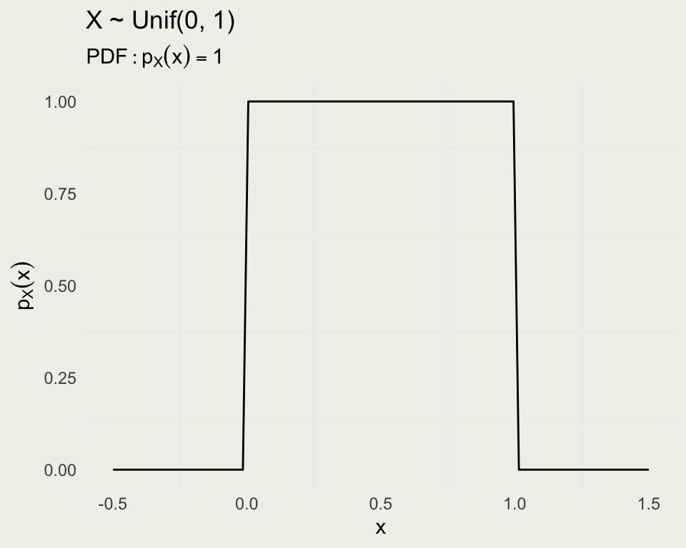
Uniform \(X \sim \text{Uniform}(\alpha, \beta)\) has the following PDF:

\[ \text{Uniform}(x|\alpha,\beta) = \frac{1}{\beta - \alpha}, \, \text{where } \alpha \in \mathbb{R} \text{ and } \beta \in (\alpha,\infty) \]

  • Your Turn: Guess the \(\E(X)\)
  • Now derive \(\E(X)\) using the definition of the Expected Value: \(\E(X) = \int x f_X(x)\, dx\)
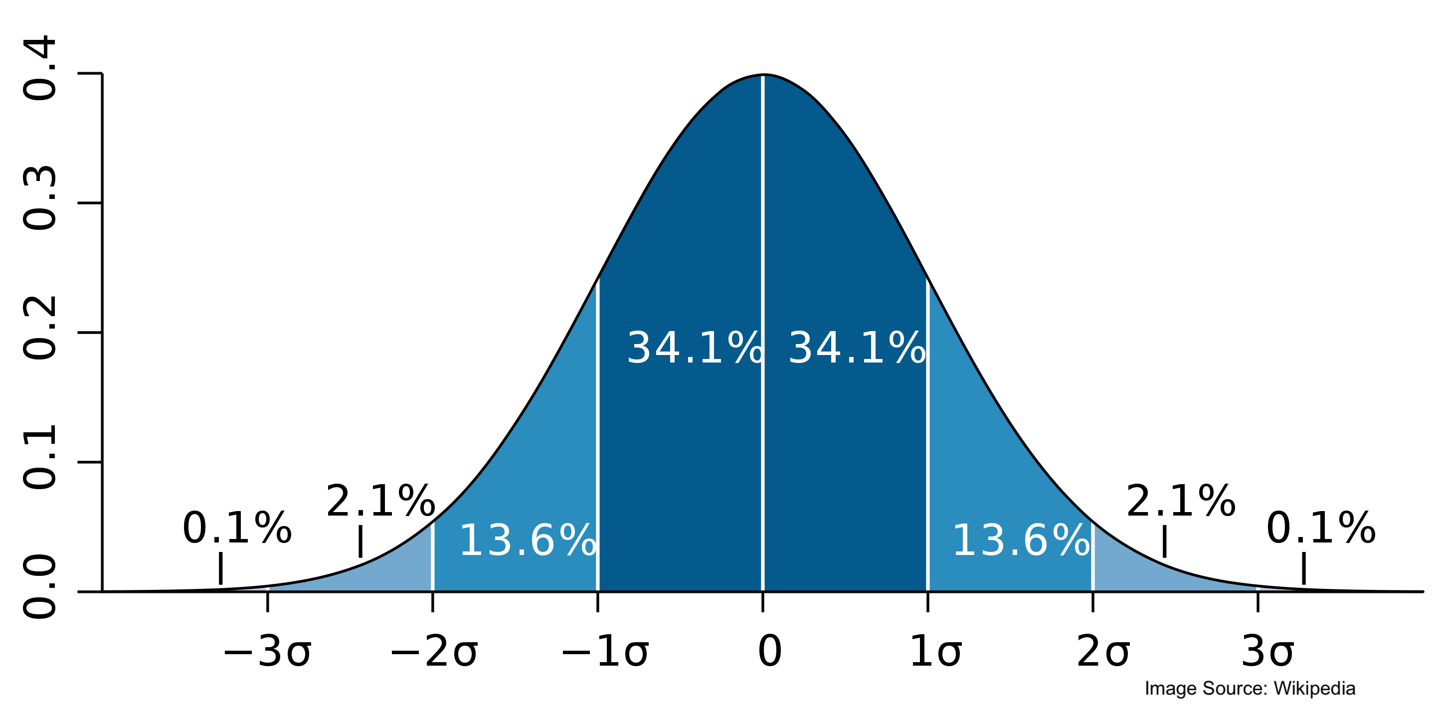
x <- seq(-0.5, 1.5, length = 100)
pdf_x <- dunif(x, min = 0, max = 1)
p <- ggplot(data.frame(x, pdf_x), aes(x, pdf_x))
p + geom_line() + ylab(expression(p[X](x))) +
  ggtitle("X ~ Unif(0, 1)", subtitle = expression(PDF: p[X](x) == 1))

Example: Stick breaking

  • You break a unit-length stick at a random point
  • Let \(X\) be the breaking point so \(X \sim \text{Uniform}(0, 1)\)
  • Let \(Y\) be the larger piece. What is \(\E(Y)\)?
  • LOTUS, says that we do not need \(f_Y\), we can work with \(f_X\)

\[ \E(Y)= \int y(x) f_X(x) dx \]

  • This works only if \(Y\) is a function of \(X\). Here, \(Y = \max\{X, 1 - X\}\).
  • We consider two cases: when \(x\) is larger than \(1/2\), \(y(x)\) is between \(1/2\) and \(1\) and when \(1 - x\) is larger, it is between \(0\) and \(1/2\):

\[ y(x) = \left\{ \begin{array}{ll} x & \text{if } 1/2 < x < 1, \text{ and} \\ 1 - x & 0 < x < 1/2 \end{array} \right. \]

  • In other words, \(\E(Y)\) can be computed as the sum of two integrals:

\[ \E(Y) = \int_{0}^{1} y(x) f_X(x)\, dx = \\ \int_{1/2}^{1} x \cdot 1 \, dx + \int_{0}^{1/2} (1-x) \cdot 1 \, dx = \\ \frac{x^2}{2} \Biggr|_{1/2}^{1} + \frac{1}{2} - \frac{x^2}{2} \Biggr|_{0}^{1/2} = \frac{3}{4} \]

  • Let’s do a quick simulation in R
x <- runif(1e4, min = 0, max = 1) # pick a random breaking point on (0, 1)
y <- ifelse(x > 0.5, x, 1 - x)    # generate y = max(x, 1-x)
mean(y) |> round(3)               # estimate the expectation E(Y)
[1] 0.75

Normal RV

  • \(X \sim \text{Normal}(\mu, \sigma)\) has the following PDF:

\[ \text{Normal}(x \mid \mu,\sigma) = \frac{1}{\sqrt{2 \pi} \ \sigma} \exp\left( - \, \frac{1}{2} \left( \frac{x - \mu}{\sigma} \right)^2 \right) \! \]

  • The bell shape comes from the \(\exp(-x^2)\) part

  • The expected value is \(\E(X) = \mu\), the mode (highest peak) and median are also \(\mu\).

  • Variance is \(\V(X) = \sigma^2\) and standard deviation \(\text{sd} = \sigma\)

  • A Normal RV can be converted to standard normal by subtracting \(\mu\) and dividing by \(\sigma\)

\[ \text{Normal}(x \mid 0, 1) \ = \ \frac{1}{\sqrt{2 \pi}} \, \exp \left( \frac{-x^2}{2} \right)\ \]

  • Sums of small contributions tend to have a normal distribution
  • Heights of people stratified by gender is a good example
  • The following data come from “Teaching Statistics, A Bag of Tricks” by Gelman and Nolan
mu_m <- 69.1   # mean heights of US males in inches
sigma_m <- 2.9 # standard deviation for same
mu_w <- 63.7   # mean heights of US women in inches
sigma_w <- 2.7 # standard deviation of the same

x <- seq(50, 80, len = 1e3)
pdf_m <- dnorm(x, mean = mu_m, sd = sigma_m)
pdf_w <- dnorm(x, mean = mu_w, sd = sigma_w)
p <- ggplot(data.frame(x, pdf_m, pdf_w), aes(x, pdf_m))
p <- p + geom_line(size = 0.2, color = 'red') + 
  geom_line(aes(y = pdf_w), size = 0.2, color = 'blue') +
  xlab("Height (in)") + ylab("") +
  ggtitle("Distribution of heights of US adults") +
  annotate("text", x = 73.5, y = 0.10, label = "Men", color = 'red') +
  annotate("text", x = 58, y = 0.10, label = "Women", color = 'blue') +
  theme(axis.text.y = element_blank(),
        axis.ticks.y = element_blank())

print(p)

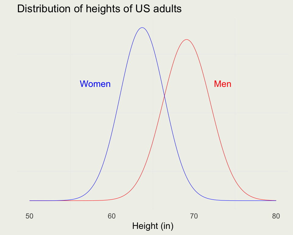
  • The combined distribution is not Normal:

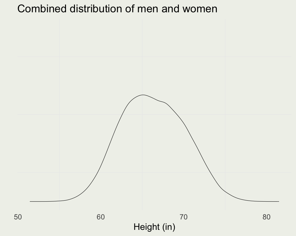
  • You randomly sample a man from the population. What is \(\P(\text{Height}_m < 65)\)
integrate(dnorm, lower = -Inf, upper = 65, 
          mean = mu_m, sd = sigma_m)$value |>
  round(2)
[1] 0.08
  • You randomly sample a woman from the population. What is \(\P(60 < \text{Height}_w < 70)\)
integrate(dnorm, lower = 60, upper = 70, 
          mean = mu_w, sd = sigma_w)$value |>
  round(2)
[1] 0.9
(integrate(dnorm, lower = -Inf, upper = 70, 
          mean = mu_w, sd = sigma_w)$value - 
integrate(dnorm, lower = -Inf, upper = 60, 
          mean = mu_w, sd = sigma_w)$value) |>
  round(2)
[1] 0.9
  • What is the probability that a randomly chosen man is taller than a randomly chosen woman?

  • We have two distributions \(M \sim \text{Normal}(\mu_m, \sigma_m)\) and \(W \sim \text{Normal}(\mu_w, \sigma_w)\). We want \(\P(M > W) = P(Z > 0),\, \text{where }Z = M - W\)

  • Sum of two normals is normal where both means and variances sum:

\[ \begin{eqnarray} Z & \sim & \text{Normal}(\mu_m + \mu_w,\, \sigma_m^2 + \sigma_m^2) \\ E(Z) & = & E(M - W) = E(M) - E(W) = 69.1 - 63.7 = 5.4 \\ \text{Var}(Z) & = & \text{Var}(M - W) = \text{Var}(M) + \text{Var}(W) = 2.9^2 + 2.7^2 = 15.7 \\ \text{sd} & = & \sqrt{Var} = \sqrt{15.7} =3.96 \\ Z & \sim & \text{Normal}(5.4, 3.96) \end{eqnarray} \]

  • To figure out when \(Z > 0\), we can integrate the PDF from 0 to Infinity:
integrate(dnorm, lower = 0, upper = Inf, 
          mean = 5.4, sd = sqrt(15.7))$value |>
  round(2)
[1] 0.91
  • We don’t have to integrate. We can evaluate the CDF instead:
1 - pnorm(0, mean = 5.4, sd = sqrt(15.7)) |>
  round(2)
[1] 0.91
  • By symmetry, the probability that a randomly chosen woman is taller than a randomly chosen man is 0.09

  • How can we check the analytic solution? We can do a simulation!

n <- 1e5
taller_m <- numeric(n)
for (i in 1:n) {
  height_m <- rnorm(1, mu_m, sigma_m)
  height_w <- rnorm(1, mu_w, sigma_w)
  taller_m[i] <- height_m > height_w
}
mean(taller_m) |> round(2)
[1] 0.91
  • Suppose you wanted to compute the variance this way. How would you do it?

What We Did Not Cover

  • Joint, Marginal, and Conditional P[M/D]Fs
  • Covariance and correlation
  • Conditional Expectations