SMaC: Statistics, Math, and Computing

Applied Statistics for Social Science Research

Eric Novik | Summer 2024 | Session 5

Session 5 Outline

• Random variables
• Bernoulli, Binomial, Geometric
• PDF and CDF
• LOTUS
• Poisson
• Expectations, Variance
• St. Petersburg Paradox
• Normal

\[ \DeclareMathOperator{\E}{\mathbb{E}} \DeclareMathOperator{\P}{\mathbb{P}} \DeclareMathOperator{\V}{\mathbb{V}} \DeclareMathOperator{\L}{\mathscr{L}} \DeclareMathOperator{\I}{\text{I}} \]

Random Variables are Not Random

• Story
• Picture

• It would be inconvenient to enumerate all possible events to describe a stochastic system

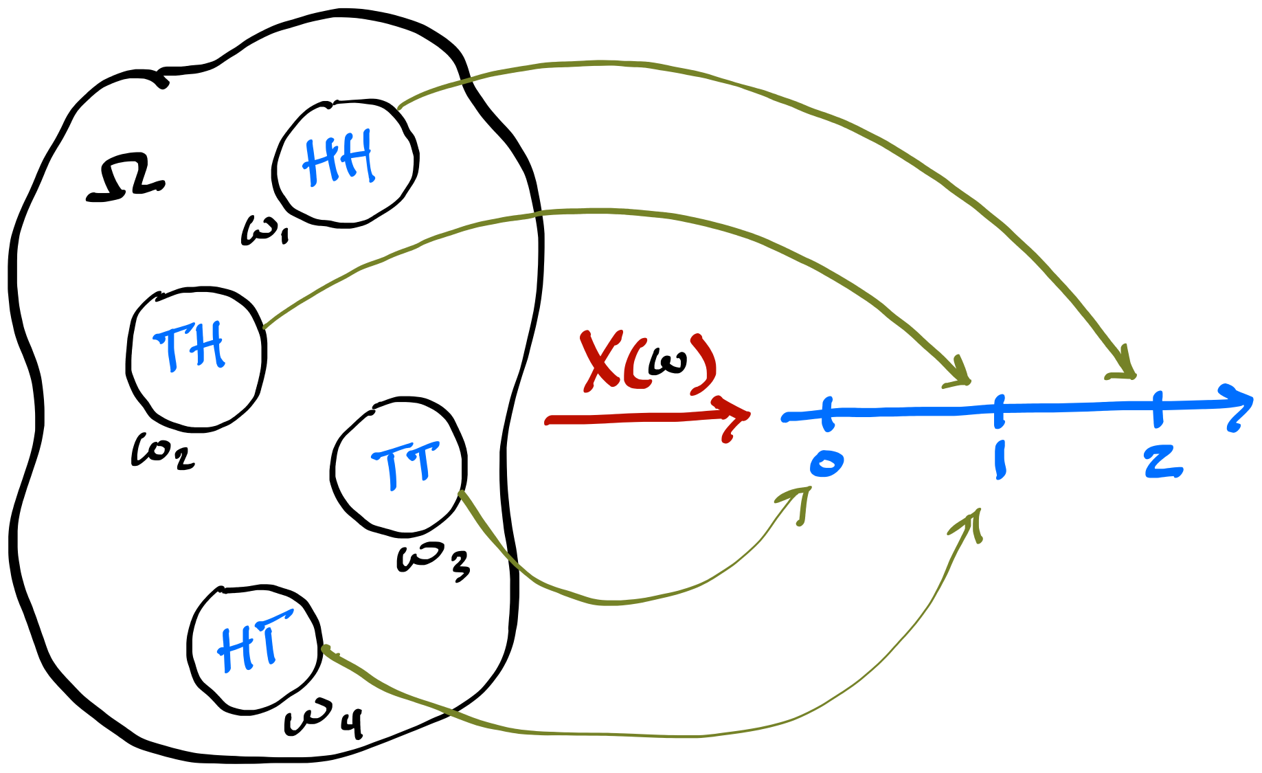
• A more general approach is to introduce a function that maps sample space \(S\) onto the Real line

• For each possible outcome \(s\), random variable \(X(s)\) performs this mapping

• This mapping is deterministic. The randomness comes from the experiment, not from the random variable (RV)

• While it makes sense to talk about \(\P(A)\), where \(A\) is an event, it does not make sense to talk about \(\P(X)\), but you can say \(\P(X(s) = x)\), which we usually write as \(\P(X = x)\)

• Let \(X\) be the number of Heads in two coin flips. You flip the coin twice, and you get \(HH\). In this case, \(s = {HH}\), \(X(s) = 2\), while \(S = \{TT, TH, HT, HH\}\)

• Random variable \(X\) for the number of Heads in two flips

Characterising Random Variables

• Introduction
• R Conventions

• Two ways of describing an RV are CDF (Cumulative Distribution Function) and PMF (Probability Mass Function) for discrete RVs and PDF (Probability Density Function) for continuous RVs. There are other ways, but we will stick with CDF and P[D/M]F.
• CDF \(F_X(x)\) is a function of \(x\) and is bounded between 0 and 1:

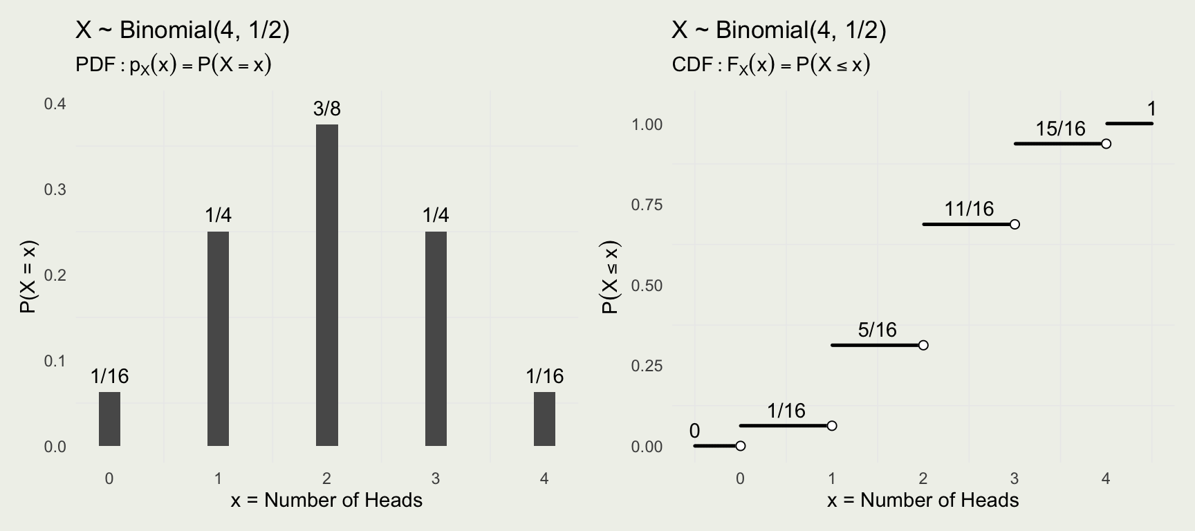
\[ F_X(x) = \P(X \leq x) \]

• PMF (for discrete RVs only) \(f_X(x)\) is a function of \(x\)

\[ f_X(x) = \P(X = x) \]

• You can get from \(f_X\) to \(F_X\) by summing. Let’s say \(x = 4\). In that case:

\[ F_X(4) = \P(X \leq 4) = \sum_{i = 4,3,2,...}\P(X = i) \]

• In R, PMFs and PDFs start with the letter d. For example dbinom() and dnormal() refer to binomial PMF and normal PDF

• CDFs start with p, so pbinom() and pnorm()

• Inverse CDFs or quantile functions, start with q so qbinom() and so on

• Random number generators start with r, so rbinom()

• A binomial RV, which we will define later, represents the number of successes in N trials. In R, the PMF is dbinom() and CDF is pbinom()

• Here is the full function signature: dbinom(x, size, prob, log = FALSE)

  • x is the number of successes, size is the number of trials N, prob is the probability of success in each trial \(\theta\), and log is a flag asking if we want the results on the log scale.

Binomial RV

• Binomial PMF
• PMF and CDF Plots
• Code to Generate the Plots

• Bernoulli RV is one coin flip with a set probability of success (say Heads)

• If \(X \sim \text{Bernoulli}(\theta)\), the PMF can be written directly as \(\P(X = x) = \theta^x (1 - \theta)^{1-x}, \, x \in \{0, 1\}\)

• Binomial can be thought of as the sum of \(N\) independent Bernoulli trials. We can also write:

\[ \text{Bernoulli}(x~|~\theta) = \left\{ \begin{array}{ll} \theta & \text{if } x = 1, \text{ and} \\ 1 - \theta & \text{if } x = 0 \end{array} \right. \]

• We can write the Binomial PMF, \(X \sim \text{Binomial}(N, \theta)\) this way:

\[ \text{Binomial}(x~|~N,\theta) = \binom{N}{x} \theta^x (1 - \theta)^{N - x} \]

\(\text{Binomial}(x~|~N=4,\theta = 1/2)\)

library(patchwork)
library(MASS)

N <- 4 # Number of successes out of x trials

# compute and plot the PMF
pmf <- dbinom(x = 0:N, size = N, prob = 1/2)
d <- data.frame(x =  0:N, y = pmf)
p1 <- ggplot(d, aes(x, pmf))
p1 <- p1 + geom_col(width = .2) + 
  geom_text(aes(label = fractions(pmf)), nudge_y = 0.02) +
  ylab("P(X = x)") + xlab("x = Number of Heads") +
  ggtitle("X ~ Binomial(4, 1/2)",
          subtitle = expression(PDF: p[X](x) == P(X == x)))

# compute and plot the CDF
x <- seq(-0.5, 4.5, length = 500)
cdf <- pbinom(q = x, size = N, prob = 1/2)
d <- data.frame(q = x, y = cdf)
dd <- data.frame(x = seq(-0.5, 4.5, by = 1), cdf = unique(cdf), x_empty = 0:5)
p2 <- ggplot(d, aes(x, cdf)) 
p2 <- p2 + geom_point(size = 0.2) + 
  geom_text(aes(x, cdf, label = fractions(cdf)), data = dd, nudge_y = 0.05) +
  geom_point(aes(x_empty, cdf), data = dd[-6, ], size = 2, color = 'white') +
  geom_point(aes(x_empty, cdf), data = dd[-6, ], size = 2, shape = 1) +
  ggtitle("X ~ Binomial(4, 1/2)",
          subtitle = expression(CDF: F[X](x) == P(X <= x))) +
  ylab(expression(P(X <= x))) + xlab("x = Number of Heads")

p1 + p2

Binomial in R

# What is the probability of getting 2 Heads out of 5 fair trials?
N <- 5; x <- 2
dbinom(x = x, size = N, prob = 0.5) |> fractions()

[1] 5/16

# What is the binomial PMF: P(X = x), for N = 5, p = 0.5?
N <- 5; x <- -2:7 # notice we range x over any integers
dbinom(x = x, size = N, prob = 0.5) |> fractions()

 [1]    0    0 1/32 5/32 5/16 5/16 5/32 1/32    0    0

# Verify that the PMF sums to 1
sum(dbinom(x = x, size = N, prob = 0.5))

[1] 1

# What is the probability of 3 heads or fewer
pbinom(3, size = N, prob = 0.5) |> fractions()

[1] 13/16

# compute the CDF: P(X <= x), for N = 5, p = 0.5
pbinom(x, size = N, prob = 0.5) |> fractions()

 [1]     0     0  1/32  3/16   1/2 13/16 31/32     1     1     1

# get from the PMF to CDF; cumsum() is the cumulative sum function
dbinom(x = x, size = N, prob = 0.5) |> cumsum() |> fractions()

 [1]     0     0  1/32  3/16   1/2 13/16 31/32     1     1     1

• Your Turn: Suppose the probability of success is 1/3, N = 10. What is the probability of 6 or more successes? Compute it with a PMF first and verify with the CDF.