SMaC: Statistics, Math, and Computing

Applied Statistics for Social Science Research

Eric Novik | Summer 2024 | Session 6

Session 6 Outline

  • Vectors and vector arithmetic
  • Matrices and matrix arithmetic
  • Determinants
  • Matrix inverses
  • Solving linear systems

\[ \DeclareMathOperator{\E}{\mathbb{E}} \DeclareMathOperator{\P}{\mathbb{P}} \DeclareMathOperator{\V}{\mathbb{V}} \DeclareMathOperator{\L}{\mathscr{L}} \DeclareMathOperator{\I}{\text{I}} \]

Introduction to Vectors

  • Linear Algebra offers a language for manipulating n-dimensional objects
  • Vectors are the basic building block of Linear Algebra
  • A straightforward way to think about them is as a column of numbers
  • How we interpret the entries is up to us
  • Vectors are typically written in a column form:
\[\begin{aligned} V = \left[\begin{matrix}a\\b\\c\end{matrix}\right] \end{aligned}\]
  • If we want the row version, we transpose it:
\[\begin{aligned} V^T = \left[\begin{matrix}a & b & c\end{matrix}\right] \end{aligned}\]

Introduction to Vectors

  • In R, vectors, unfortunately, are neither row nor column vectors
  • R makes some assumptions when performing vector-matrix arithmetic
  • We already saw lots of vectors whenever we used c() function or generated random numbers with, say runif() function
set.seed(123)
(v <- c(sample(3)))
[1] 3 1 2
class(v)
[1] "integer"
  • R reports the \(v\) is an integer vector

  • You can add two vectors in a usual way, elementwise:

\[\begin{aligned} \left[\begin{matrix}3\\1\\2\end{matrix}\right]+\left[\begin{matrix}2\\1\\3\end{matrix}\right]=\left[\begin{matrix}5\\2\\5\end{matrix}\right] \end{aligned}\]
  • In R:
v
[1] 3 1 2
w
[1] 2 1 3
v + w
[1] 5 2 5

Introduction to Vectors

  • You can take linear combination \(av + bw\), where a and b are scalars
2*v + 3*w # linear combination
[1] 12  5 13
  • You can also take dot product: \(v \cdot w\), which results in a scalar
\[\begin{aligned} v \cdot w = \left[\begin{matrix}3 & 1 & 2\end{matrix}\right]\left[\begin{matrix}2\\1\\3\end{matrix}\right]=\left[\begin{matrix}13\end{matrix}\right] \end{aligned}\]
  • In R, we multiply vectors and Matrices with %*%, not *, which will produce a component-wise multiplication, not a dot product
v %*% w # dot product
     [,1]
[1,]   13
v * w   # component wise multiplication
[1] 6 1 6
  • We write dot product this way:

\[ v^T w = v_1w_1 + v_2w_2 + \cdots + v_nw_n \]

Introduction to Vectors

  • When is dot product zero?
v <- c(1, 1)
w <- c(1, -1)
v %*% w
     [,1]
[1,]    0
(3 * v) %*% (4 * w)
     [,1]
[1,]    0
  • These vectors are perpendicular (orthogonal)

Introduction to Vectors

  • A length of a vector is the square root of the dot product with itself

\[ ||v|| = \sqrt{v \cdot v} = \sqrt{v_1^2 + v_2^2 + \cdots v_n^2} \]

v <- c(1, 1)  
sqrt(v %*% v) # this is sqrt of 2 
         [,1]
[1,] 1.414214

Introduction to Matrices

  • You can think of a matrix as a rectangular (or square) set of numbers
  • \(m{\times}n\) matrix has m rows and n columns
  • In statistics, it is convenient to think of a matrix as n columns where each column is a variable like the price of the house, and the rows are the observations for each house
  • In Linear Algebra books, you will often see linear equations written as \(Ax = b\), where we are trying to find \(x\)
  • In statistics, we usually write the same thing as \(X\beta = y\), and we are trying to find \(\beta\)
  • Another source of confusion: matrix \(A\) is sometimes called a coefficient matrix in Linear Algebra books. In statistics, the entries in \(A\) (the \(X\) matrix) have observations, and the \(\beta\) vector contains coefficients estimated from A and b (X and y).

Introduction to Matrices

  • A good way to think about the Matrices is that they act on vectors and transform them in some way (stretch or turn them)
  • You can think of this transformation as encoding the eventual locations of the basis vectors
  • Standard basis vectors in \(R^2\) (two-dimensional space), are commonly called \(\hat{i}\) with location \((1, 0)\), and \(\hat{j}\) with location \((0, 1)\).
  • Notice their dot product is zero: \(\hat{i} \cdot \hat{j} = 0\) and so they are orthogonal
  • Let’s look at one simple transformation – rotation by 90 degrees counter-clockwise
  • Recall, vectors \(v\) and \(w\):

\[ v = \left[ \begin{matrix}1\\2\end{matrix} \right] w = \left[ \begin{matrix}3\\1\end{matrix} \right] \]

  • The following matrix encodes a 90-degree, counterclockwise rotation. Why?

\[ R = \begin{bmatrix} 0 & -1 \\ 1 & 0 \end{bmatrix} \]

  • Let’s see how this matrix will act on vectors \(v\) and \(w\). That’s where multiplication comes in.

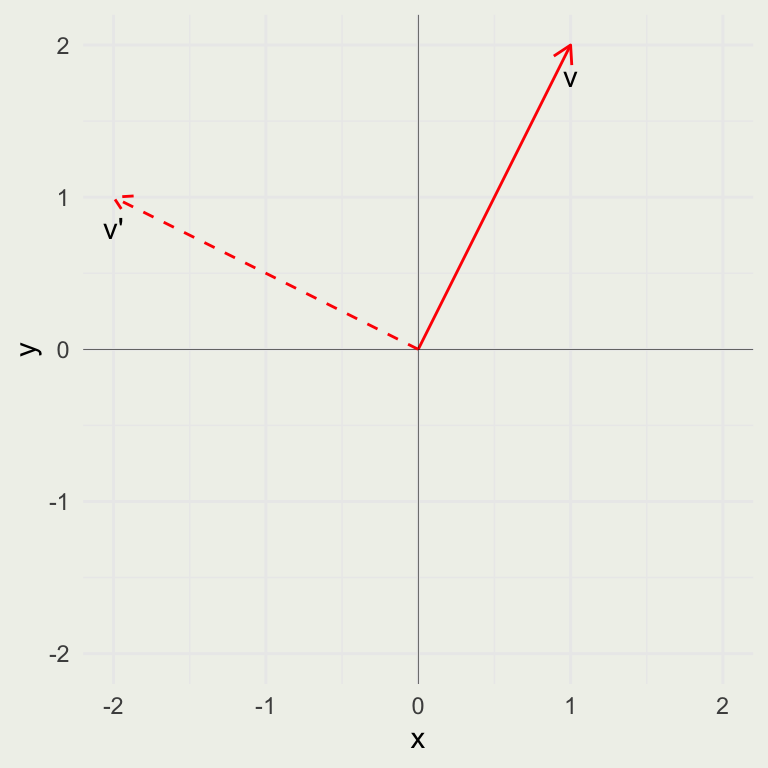
\[ Rv = \begin{bmatrix} 0 & -1 \\ 1 & 0 \end{bmatrix} \begin{bmatrix} 1 \\ 2 \end{bmatrix} = 1 \begin{bmatrix} 0 \\ 1 \end{bmatrix} + 2 \begin{bmatrix} -1 \\ 0 \end{bmatrix} = \begin{bmatrix} 0 \\ 1 \end{bmatrix} + \begin{bmatrix} -2 \\ 0 \end{bmatrix} = \begin{bmatrix} -2 \\ 1 \end{bmatrix} \]

  • We scale the first vector, then scale the second, and then add.
  • The following shows the same operation you can do in one step in R.
R <- matrix(c(0, 1, -1, 0), ncol = 2)
R
     [,1] [,2]
[1,]    0   -1
[2,]    1    0
v <- c(1, 2)
(v_prime <- R %*% v)
     [,1]
[1,]   -2
[2,]    1
  • Now let’s plot \(v\) and \(v'\). Notice, the 90 degree rotation

Matrix Multiplication

  • Our matrix encodes a rotation of every single vector in \(R^2\).
  • In particular, it rotates every point \((x, y)\) in \(R^2\) by 90 degrees
  • We can do this transformation in one go by applying the Rotation matrix to another matrix comprising our vectors \(v\) and \(w\)
  • The number of columns in the Rotation matrix has to match the number of rows in the \(K = [v, w]\) matrix
(K <- matrix(c(v, w), ncol = 2))
     [,1] [,2]
[1,]    1    3
[2,]    2    1
(K_prime <- R %*% K)
     [,1] [,2]
[1,]   -2   -1
[2,]    1    3
  • The resulting matrix \(K\), has the correctly rotated \(v\) in the first column and rotated \(w\) in the second column.

  • Another way to think about this operation is to encode two transformations in \(K'\) — the \(K\) transformation followed by the \(R\) transformation. We can now use the resulting \(K'\) matrix and apply these two transformations in one swoop to any vector in \(R^2\).

  • Think about why matrix multiplication, in general, does not commute — \(RK \neq KR\)

  • Rotating red (\(v = [1 \ 2]\)) and blue (\(w = [3 \ 1]\)) vectors by 90 degrees

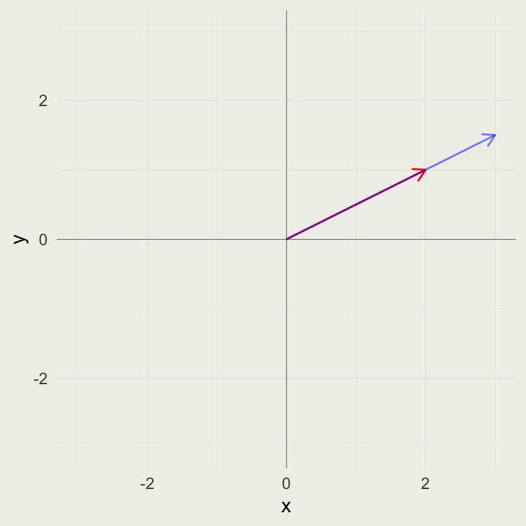
  • Your Turn: Come up with a 90-degree clockwise rotation matrix and show that it sends \((2, 2)\) to \((2, -2)\)

  • Now pick three vectors in \(R^2\) and rotate all three at the same time

Linear Independence and Determinants

  • Think of a determinant as a (signed) area scaling factor from the basis \((\hat{i}, \hat{j})\) to the transformed vectors
  • The area represented by two \(R^2\) basis vectors is 1
# this matrix scales the area by 12
(X <- matrix(c(4, 0, 0, 3), ncol = 2))
     [,1] [,2]
[1,]    4    0
[2,]    0    3
# compute the determinant
det(X)
[1] 12
  • What happens if the columns of \(X\) are linear combinations of each other?
  • Geometrically, that means that in \(R^2\), they both sit on the same line
# the second column is the first column * 1.5
(X <- matrix(c(2, 1, 1.5 * 2, 1.5 * 1), ncol = 2))
     [,1] [,2]
[1,]    2  3.0
[2,]    1  1.5
# compute the determinant
det(X)
[1] 0

Example: Random Matrix

  • Generate a random, say 5x5 matrix
  • Is it likely that we will get linearly dependent columns?
set.seed(123)
(X <- matrix(sample(25), ncol = 5))
     [,1] [,2] [,3] [,4] [,5]
[1,]   15   18    9   25    2
[2,]   19   11   21   17   16
[3,]   14    5   24    1    7
[4,]    3   23   20   12    8
[5,]   10    6   22   13    4
det(X)
[1] 1155943
  • This is a full rank matrix that encodes a transformation in \(R^5\) — 5-dimensional space

Computing Determinants

  • Don’t bother doing it by hand
\[\begin{aligned} A = \left[\begin{matrix}a & c\\b & d\end{matrix}\right] \end{aligned}\] \[\begin{aligned} \det(A) = a d - b c \end{aligned}\] \[\begin{aligned} B = \left[\begin{matrix}a & d & g\\b & e & h\\c & f & i\end{matrix}\right] \end{aligned}\] \[\begin{aligned} \det(B) = a e i - a f h - b d i + b f g + c d h - c e g \end{aligned}\]

Linear Systems and Inverses

  • One of the key ideas from Linear Algebra that is relevant to statistics is solving linear systems
  • This is where estimating coefficients in \(X\beta = y\) comes from
  • If \(X\) is a square matrix, the problem is not statistical but algebraic
  • The reason is that if we have the same number of equations as we have unknowns, we can solve the system exactly unless X is not full rank
  • For example, try to solve this system:

\[ 2x + y = 1 \\ 4x + 2y = 1 \]

  • Question: Geometrically, what does it mean to solve a system of equations?
  • You should now have a deeper understanding of why there is no solution
(A <- matrix(c(2, 4, 1, 2), ncol = 2))
     [,1] [,2]
[1,]    2    1
[2,]    4    2
det(A)
[1] 0
  • Before we talk about overdetermined systems (more equations than unknowns) that we see in statistics, let’s see how it works in the square matrix case
  • To see what a matrix inverse does, let’s bring back the 90-degree counterclockwise rotation matrix \(A\)
\[\begin{aligned} A = \left[\begin{matrix}0 & -1\\1 & 0\end{matrix}\right] \end{aligned}\]
  • The idea of an inverse is to reverse the action of this transformation
  • In this case, we need a clockwise 90-degree rotation matrix
  • We can find that matrix by directly tracing the basis vectors
\[\begin{aligned} A^{-1} = \left[\begin{matrix}0 & 1\\-1 & 0\end{matrix}\right] \end{aligned}\]
  • Let’s check our results in R. When you multiply a matrix by its inverse, you get back the identity matrix (which is like when you divide a scalar by its reciprocal, you get 1)
(A <- matrix(c(0, 1, -1, 0), 2, 2))
     [,1] [,2]
[1,]    0   -1
[2,]    1    0
(A_inv <- matrix(c(0, -1, 1, 0), 2, 2))
     [,1] [,2]
[1,]    0    1
[2,]   -1    0
A_inv %*% A
     [,1] [,2]
[1,]    1    0
[2,]    0    1
# find an inverse using R's solve function
solve(A)
     [,1] [,2]
[1,]    0    1
[2,]   -1    0
  • We are now ready to solve the square linear system \(Ax = b\), in the case when A is full rank

\[ \begin{eqnarray} Ax & = & b \\ A^{-1}Ax & = & A^{-1}b \\ x & = & A^{-1}b \end{eqnarray} \]

  • The general solution in two-dimensional case:
\[\begin{aligned} \left[\begin{matrix}a & c\\b & d\end{matrix}\right]x = \left[\begin{matrix}b_{1}\\b_{2}\end{matrix}\right] \end{aligned}\] \[\begin{aligned} \det(A) = a d - b c \end{aligned}\] \[\begin{aligned} A^{-1} = \left[\begin{matrix}\frac{d}{a d - b c} & - \frac{c}{a d - b c}\\- \frac{b}{a d - b c} & \frac{a}{a d - b c}\end{matrix}\right] \end{aligned}\] \[\begin{aligned} x = \left[\begin{matrix}\frac{b_{1} d - b_{2} c}{a d - b c}\\\frac{a b_{2} - b b_{1}}{a d - b c}\end{matrix}\right] \end{aligned}\]
  • In R, solve(A) inverts the matrix, and solve(A, b) solves \(Ax = b\).
(A <- matrix(sample(9), ncol = 3))
     [,1] [,2] [,3]
[1,]    3    1    7
[2,]    4    9    2
[3,]    6    5    8
(b <- c(1, 2, 3))
[1] 1 2 3
solve(A, b) %>% round(2)
[1]  0.93 -0.14 -0.24
# same as above
solve(A) %*% b %>% round(2)
      [,1]
[1,]  0.93
[2,] -0.14
[3,] -0.24

Your Turn

  • Consider the following system of equations:

\[ \begin{eqnarray} 3x + 2y + 1.5z & = & 4 \\ 7x + y & = & 2 \\ 3y + 2z & = & 1 \end{eqnarray} \]

  • Express it in matrix form, solve it in R using the solve() function, and validate that the results are correct

Some Useful Rules

If you put on socks and then shoes, the first to be taken off are the ____

— Gilbert Strang (discussing the order of undoing the inverse)

\[ (ABC \dots)^{-1} = \dots C^{-1}B^{-1}A^{-1} \\ (A^T)^{-1} = (A^{-1})^T \\ (A + B)^T = A^T + B^T \\ (ABC \dots)^T = \dots C^T B^T A^T \]

Solving n > p Systems

  • Frequentist statistical inference is concerned with “solving” overdetermined systems
  • We have lots of observations with relatively few variables. (Sometimes, we have more variables than observations, but we will not discuss it here)
  • Clearly, there is no exact solution
  • In fact, there are typically infinitely many ways in which you can draw a line through a cloud of points or a plane through n-dimensional space
  • Optimization based (or frequentist) inference is concerned with finding the most likely values of the unknowns giving rise to that line (or plane) and approximating their variance
  • Integration based (or Bayesian) inference is concerned with finding a joint PDF of the unknowns – all plausible values weighted by their probability. Therefore, the “estimated variance” is a consequence of this PDF. (Recall our example of estimating variance from the distribution of the difference in heights.) In this sense, Bayesian inference is an uncertainty-preserving system, a very desirable quality.
  • For simple linear models, both of these methods produce similar results.

Solving an Overdetermined \(X\hat{\beta} = y\)

  • We are switching to a more familiar (to statisticians) notation of \(X \beta = y\) (instead of \(Ax = b\))
  • We typically augment the \(X\) matrix with the column of 1s on the left to model the intercept term, sometimes called \(\beta_0\)
  • This should make sense when you think about \(X \beta\) as the linear combination of columns of \(X\)
  • In this form, \(X\) is usually called the design matrix or the model matrix
  • The problem is that \(X\) is not invertible, even if columns of \(X\) are linearly independent
  • Let’s say that \(X\) is a \(3 \times 2\) matrix (3 rows and 2 columns), and columns are linearly independent. Note that \(\beta\) is \(2 \times 1\) and \(y\) is \(3 \times 1\).
  • \(X\) and its linear combinations \(X\beta\) span a plane in three-dimensional space – there is no way for it to reach the target vector \(y\) in \(R^3\)

Approximating a Solution to Overdetermined \(X\hat{\beta} = y\)

  • If we can not reach \(y\), we need to find a vector in the column space of \(X\) that is closest (in a certain sense) to \(y\)

  • The projection of \(y\) onto this plane gives us the answer

Solving an Overdetermined \(X\hat{\beta} = y\)

  • This residual \(r\) is also called the error term
  • This error, \(y - X\hat{\beta}\), is the smallest when it’s perpendicular to the plane
  • Another way of saying that is that:

\[ X^T(y - X\hat{\beta}) = 0 \]

  • We can now solve this normal equation:

\[ \begin{eqnarray} X^T(y - X\hat{\beta}) & = & 0 \\ X^TX\hat{\beta} & = & X^Ty \\ (X^TX)^{-1}(X^TX)\hat{\beta} & = & (X^TX)^{-1}X^Ty \\ \hat{\beta} & = & (X^TX)^{-1}X^Ty \end{eqnarray} \]

  • Matrix \(X^TX\) is square and symmetric. It is also invertible if the columns of \(X\) are linearly independent:
(X <- matrix(sample(6), ncol = 2))
     [,1] [,2]
[1,]    2    1
[2,]    5    4
[3,]    3    6
(XtX <- t(X) %*% X)
     [,1] [,2]
[1,]   38   40
[2,]   40   53
solve(XtX) %>% round(2)
      [,1]  [,2]
[1,]  0.13 -0.10
[2,] -0.10  0.09
(X <- matrix(c(1, 2, 3, 2, 4, 6), ncol = 2))
     [,1] [,2]
[1,]    1    2
[2,]    2    4
[3,]    3    6
(XtX <- t(X) %*% X)  # will not invert
     [,1] [,2]
[1,]   14   28
[2,]   28   56

Motion in the Straight Line

  • Recall, from lecture 1, our example of a car moving in a straight line where we have noisy measurements of its position over time
  • At the time, we assumed we were able somehow to find the intercept and slope of the equation
  • We are now in a position to solve the problem

Motion in the Straight Line

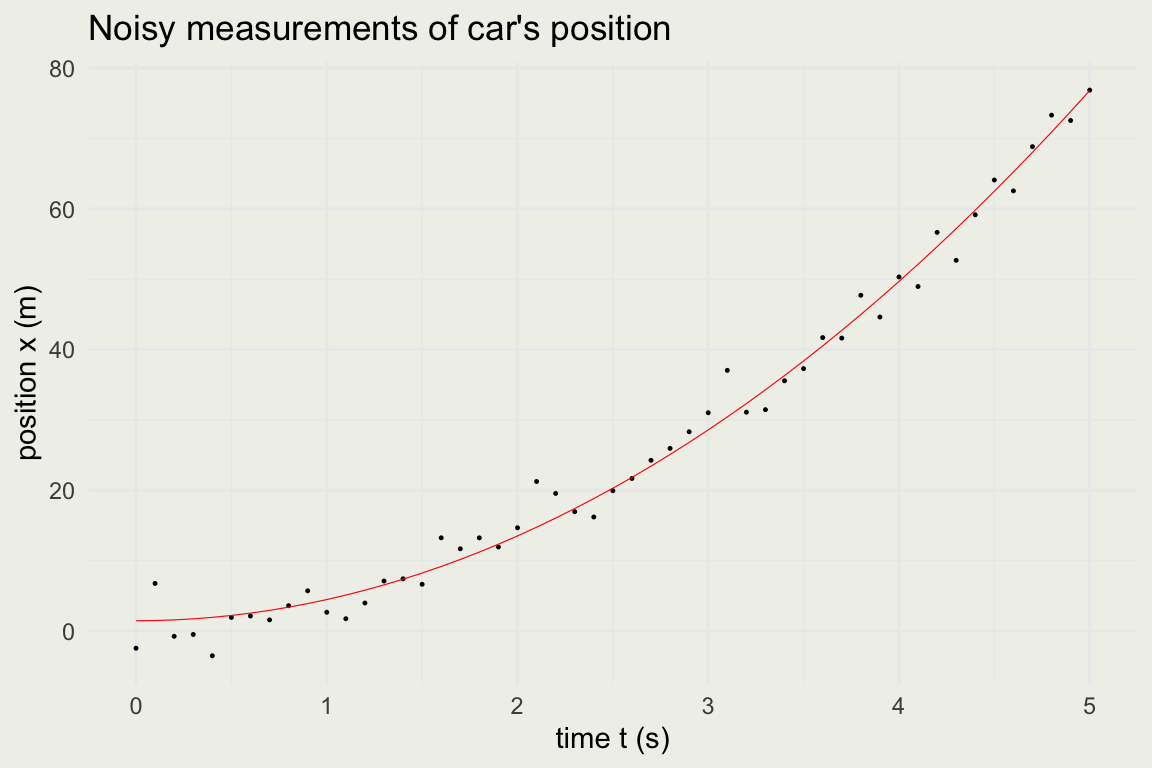
  • This is a quadratic function. How can we solve it using linear regression (the least squares method)?

  • We assumed the equation of motion was \(x(t) = a + bt^2\), which we will write as \(y(t) = \beta_0 + \beta_1 t^2\)

  • The unknowns are \(\beta_0\) and \(\beta_1\)

  • Let’s express it in the matrix notation

  • What is our design matrix \(X\)? We have 51 observations, so \(X\) will have two columns and 51 rows: a column of 1s for the intercept and a column of times squared \(t^2\)

  • Our unknown vector \(\hat{\beta}\) has two elements \((\hat{\beta_0},\, \hat{\beta_1)}\)

  • \(y\) is our outcome vector of length 51, capturing the car’s position at each time point \(t\)

  • \(y = X\hat{\beta}\) captures our system in matrix form

# length of t (our time vector)
length(t)
[1] 51
# first few elements of t
head(t)
[1] 0.0 0.1 0.2 0.3 0.4 0.5
# construct the design matrix
X <- matrix(c(rep(1, length(t)), t^2), ncol = 2)
head(X)
     [,1] [,2]
[1,]    1 0.00
[2,]    1 0.01
[3,]    1 0.04
[4,]    1 0.09
[5,]    1 0.16
[6,]    1 0.25
# inspect the vector y
length(y)
[1] 51
head(y)
[1] -2.4417028  6.7615084 -0.7502334 -0.4900157 -3.5129263  1.9331119
  • Recall, that the least squares estimate of \(\beta\) is given by \(\hat{\beta} = (X^TX)^{-1}X^Ty\)
beta_hat <- solve(t(X) %*% X) %*% t(X) %*% y
beta_hat %>% round(2)
     [,1]
[1,] 1.46
[2,] 3.01
data <- data.frame(y = y, t_squared = t^2)
# compare to R's lm()
fit <- lm(y ~ t_squared, data = data)
arm::display(fit)
lm(formula = y ~ t_squared, data = data)
            coef.est coef.se
(Intercept) 1.46     0.54   
t_squared   3.01     0.05   
---
n = 51, k = 2
residual sd = 2.60, R-Squared = 0.99
  • Warning: do not use \((X^TX)^{-1}X^Ty\) directly as above; it’s computationally inefficient
d <- data.frame(yhat = beta_hat[1] + beta_hat[2] * x^2)
p + geom_line(aes(y = yhat), data = d, size = 0.2, color = 'red')

Your Turn

  • Look at the dataset mtcars
  • Plot mpg against wt, treating mpg as the output variable \(y\). (We generally don’t like to use the words dependent vs. independent in this context)
  • Using the normal equations, find the intercept and slope of the best-fit line
  • Validate that it matches the output from lm
  • Now plot the line over the data and see if it “fits”