SMaC: Statistics, Math, and Computing

Applied Statistics for Social Science Research

Eric Novik | Summer 2024 | Session 7

Session 7 Outline

Statistical inference
Sampling distribution
Standard errors
Confidence intervals
Degrees of freedom and t distribution
Bias and uncertainty
Statistical significance

\[ \DeclareMathOperator{\E}{\mathbb{E}} \DeclareMathOperator{\P}{\mathbb{P}} \DeclareMathOperator{\V}{\mathbb{V}} \DeclareMathOperator{\L}{\mathscr{L}} \DeclareMathOperator{\I}{\text{I}} \]

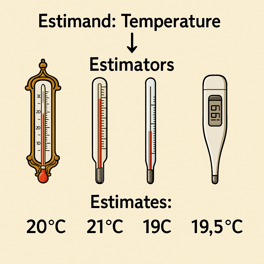
Introduction to Statistical Inference

Statistical Inference: A process of learning from noisy measurements
Key Challenges:
- Generalizing from a sample to the population of interest
- Learning what would have happened under different treatment
- Understanding the relationship between the measurement and the estimand

Image source: https://diff.healthpolicydatascience.org/

Measurement Error Models

We are trying to estimate the parameters of some data-generating process
For our car example, we assumed that the car position data are coming from the following model:

\[ x_i(t) = a + bt_i^2 + \epsilon_i \]

We also assumed that time \(t\) was observed precisely, but we can also have an error in \(t\)
Errors may be multiplicative, not just additive

Sampling Distribution

Generative model for our data: given the generative model, we can create replicas of the dataset
Sampling distribution is typically unknown and depends on the data collection, how subjects are assigned to treatment conditions, sampling process
Examples
- Simple random sample of size \(n\) from the population of size \(N\). Here, each person has the same probability of being selected
- Our constant acceleration model \(x_i(t) = a + bt_i^2 + \epsilon_i\), where we fix \(a\) and \(b\), and \(t\), and draw \(\epsilon\) from an error distribition, such as \(\text{Normal}(0, 1)\)
- We can write some code to generate observations according to this process (which is what I did for the car example)

Standard Errors

Standard error is the estimated standard deviation of the estimate
It provides a measure of uncertainty around the estimate
Standard error decreases as the sample size increases
To estimate the SE of the mean from a large population with sd = \(\sigma\): \(\frac{\sigma}{\sqrt{n}}\)

set.seed(1)
n <- 100; mu <- 5; sigma <- 1.5
x <- rnorm(n, mean = mu, sd = sigma)
x_bar <- mean(x); round(x_bar, 2)

[1] 5.16

(se <- sigma/sqrt(n))

[1] 0.15

If \(\sigma\) is unknown, we can estimate it from the sample: \(s = \sqrt{\frac{1}{n-1} \sum_{i=1}^{n} (x_i - \bar{x})^2}\)

var(x)

[1] 1.815215

sum((x - x_bar)^2) / (n - 1)

[1] 1.815215

Confidence Intervals

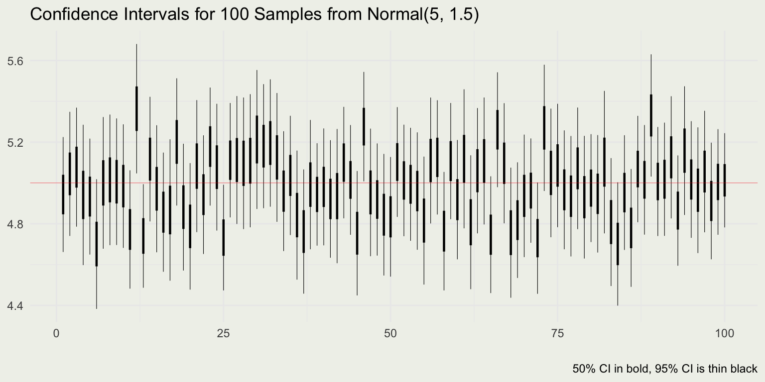
For a given sampling distribution, confidence interval provides a range of parameter values consistent with the data
For example, for a normal sampling distribution, an estimate \(\hat{\theta}\) will fall in \(\hat{\theta} \pm 2\cdot\text{se}\) about 95% of the time

Confidence Intervals for Proportions

In surveys, we are often interested in estimating the standard error of the proportion
Suppose we want to estimate the proportion of the US population that supports same-sex marriage
Say you randomly survey \(n = 500\) from the population, and \(y = 355\) people respond yes¹
The estimate of the proportion is \(\hat{\theta} = y/n\) with the \(\text{se} = \sqrt{\hat{\theta}(1 -\hat{\theta})/n }\)

n <- 500
y <- 355
theta_hat <- y/n
theta_hat |> round(2)

[1] 0.71

se <- sqrt(theta_hat * (1 - theta_hat) / n)
se |> round(2)

[1] 0.02

theta_hat + 2*se |> round(2)

[1] 0.75

theta_hat - 2*se |> round(2)

[1] 0.67

ci_95 <- theta_hat + qnorm(c(0.025, 0.975)) * se
ci_95 |> round(2)

[1] 0.67 0.75

Your Turn

In a national survey of \(n\) people, how large does \(n\) have to be so that you can estimate presidential approval to within a standard error of ±3 percentage points, ±1 percentage points?

Standard Error for Differences

We already saw an example of how to add variances from two independent RVs

\[ \text{se}_{\text{diff}} = \sqrt{\text{se}_1^2 + \text{se}_2^2} \]

Your turn: How large does \(n\) have to be so that you can estimate the gender gap in approval to within a standard error of ±3 percentage points?

Computer Demo: Computing CIs

These demos are taken from the book Active Statistics by Gelman and Vehtari

# Generate fake data
p <- 0.3
n <- 20
data <- rbinom(1, n, p)
print(data)

# Estimate proportion and calculate confidence interval
p_hat <- data / n
se <- sqrt(p_hat * (1 - p_hat) / n)
ci <- p_hat + c(-2, 2) * se
print(ci) 

# Put it in a loop
reps <- 100
for (i in 1:reps) {
  data <- rbinom(1, n, p)
  p_hat <- data / n
  se <- sqrt(p_hat * (1 - p_hat) / n)
  ci <- p_hat + c(-2, 2) * se
  print(ci) 
}

Computer Demo: Proportions, Means, and Differences of Means

# Read data from here:  https://github.com/avehtari/ROS-Examples
library("foreign")
library("dplyr")
pew_pre <- read.dta(
  paste0(
    "https://raw.githubusercontent.com/avehtari/",
    "ROS-Examples/master/Pew/data/",
    "pew_research_center_june_elect_wknd_data.dta"
  )
)
pew_pre <- pew_pre |> select(c("age", "regicert")) %>%
  na.omit() |> filter(age != 99)
n <- nrow(pew_pre)

# Estimate a proportion (certain to have registered for voting?)
registered <- ifelse(pew_pre$regicert == "absolutely certain", 1, 0)
p_hat <- mean(registered)
se_hat <- sqrt((p_hat * (1 - p_hat)) / n)
round(p_hat + c(-2, 2) * se_hat, 4) # ci

# Estimate an average (mean age)
age <- pew_pre$age
y_hat <- mean(age)
se_hat <- sd(age) / sqrt(n)
round(y_hat + c(-2, 2) * se_hat, 4) # ci

# Estimate a difference of means
age2 <- age[registered == 1]
age1 <- age[registered == 0]
y_2_hat <- mean(age2)
se_2_hat <- sd(age2) / sqrt(length(age2))
y_1_hat <- mean(age1)
se_1_hat <- sd(age1) / sqrt(length(age1))
diff_hat <- y_2_hat - y_1_hat
se_diff_hat <- sqrt(se_1_hat ^ 2 + se_2_hat ^ 2)
round(diff_hat + c(-2, 2) * se_diff_hat, 4) # ci

Degrees of Freedom

Some distributions rely on the concept of degrees of freedom
Degrees of freedom balance the need for accurate estimation against the amount of data available; it’s a way to correct for overfitting
The more parameters you estimate, the fewer degrees of freedom you have left for other calculations
The data will give us \(n\) (sample size) degrees of freedom, and \(p\) number of parameters will be used up during the estimation

Normal and t Distribution

t distribution has a degrees freedom parameter, and with a low number of degrees of freedom, it has heavier tails than the Normal

Confidence Intervals from the t Distribution

t distribution has location and scale parameters and is symmetric like the Normal
Standard error would have \(n-1\) degrees of freedom as one will be estimated to compute the mean
Suppose you threw 5 darts and the distance from bull’s eye was as follows (standard dart board radius is about 23 cm)

# Distance from the bull's eye in cm
data <- c(8, 6, 10, 5, 18)

# Calculate the sample mean
mean_data <- mean(data)

# Calculate the standard error of the mean
se_mean <- sd(data) / sqrt(length(data))

# Degrees of freedom
df <- length(data) - 1

# Calculate the 95% and 50% confidence interval 
ci_95 <- mean_data + qt(c(0.025, 0.975), df) * se_mean
ci_50 <- mean_data + qt(c(0.25, 0.75), df) * se_mean

# Output the results
mean_data |> round(2)

[1] 9.4

se_mean |> round(2)

[1] 2.32

ci_95 |> round(2)

[1]  2.97 15.83

ci_50 |> round(2)

[1]  7.69 11.11

Bias and Uncertainty

There is a lot more to it than what is in following standard picture
Discuss among yourselves what are the potential sources of bias

Statistical Significance

Comes up in NHST: Null Hypothesis Significance Testing
Bad decision filter: if p-value is less than 0.05 (relative to some Null), the results can be trusted, otherwise they are likely noise
Often, estimates (coefficients) are labeled as not significant if they are within 2 SEs: selecting models this way is also problematic
You flip a coin 10 times and observe 7 heads. Is there evidence of coin bias?
What about if you got 70 heads out of 100?

Some Problems with Statistical Significance

Statistical significance does not mean practical (or in the case of Biostats clinical) significance
No significance does not mean there is no effect
The difference between “significant” and “not significant” is not itself statistically significant
Researcher degrees of freedom, p-hacking