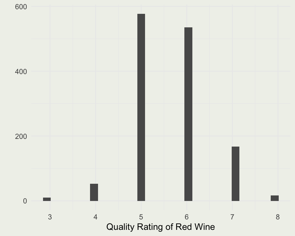
SMaC: Statistics, Math, and Computing

Applied Statistics for Social Science Research

Eric Novik | Summer 2023 | Session 07

Session 8 Outline

  • Statistical analysis workflow
  • Introduction to the rstanarm package
  • Setting up a linear regression
  • Model evaluation
  • Model expansion

\[ \DeclareMathOperator{\E}{\mathbb{E}} \DeclareMathOperator{\P}{\mathbb{P}} \DeclareMathOperator{\V}{\mathbb{V}} \DeclareMathOperator{\L}{\mathscr{L}} \DeclareMathOperator{\I}{\text{I}} \]

Analysis Workflow

  • Following is a high-level, end-to-end view from “R for Data Science” by Wickham and Grolemund

Analysis Workflow

Some Notation

  • Observed data \(y\)
  • Unobserved but observable data \(\widetilde{y}\)
  • Unobservable parameters \(\theta\)
  • Covariates \(X\)
  • Prior distribution \(f(\theta)\)
  • Likelihood (as a function of \(\theta\)), \(f(y | \theta, X)\)
  • Posterior distribution \(f(\theta | y, X)\) (for Bayesian inference only)

Bayes vs Frequentist Inference

  • Estimation is the process of figuring out the unknowns, i.e., unobserved quantities
  • In frequentist inference, the problem is framed in terms of the most likely value(s) of \(\theta\)
  • Bayesians want to characterize the whole distribution, a much more ambitious goal
  • Suppose we want to characterize the following function, which represents some distribution of the unknown parameter:

Wine Dataset

Wine Dataset

d <- read.delim("data/winequality-red.csv", sep = ";")
dim(d)
[1] 1599   12
d <- d[!duplicated(d), ] # remove the duplicates
dim(d)
[1] 1359   12
knitr::kable(head(d))
fixed.acidity volatile.acidity citric.acid residual.sugar chlorides free.sulfur.dioxide total.sulfur.dioxide density pH sulphates alcohol quality
1 7.4 0.70 0.00 1.9 0.076 11 34 0.9978 3.51 0.56 9.4 5
2 7.8 0.88 0.00 2.6 0.098 25 67 0.9968 3.20 0.68 9.8 5
3 7.8 0.76 0.04 2.3 0.092 15 54 0.9970 3.26 0.65 9.8 5
4 11.2 0.28 0.56 1.9 0.075 17 60 0.9980 3.16 0.58 9.8 6
6 7.4 0.66 0.00 1.8 0.075 13 40 0.9978 3.51 0.56 9.4 5
7 7.9 0.60 0.06 1.6 0.069 15 59 0.9964 3.30 0.46 9.4 5

Scaling the Data

ds <- scale(d) # subtract the mean and divide by sd
knitr::kable(head(ds) %>% round(2))
fixed.acidity volatile.acidity citric.acid residual.sugar chlorides free.sulfur.dioxide total.sulfur.dioxide density pH sulphates alcohol quality
1 -0.52 0.93 -1.39 -0.46 -0.25 -0.47 -0.38 0.58 1.29 -0.58 -0.95 -0.76
2 -0.29 1.92 -1.39 0.06 0.20 0.87 0.60 0.05 -0.71 0.12 -0.58 -0.76
3 -0.29 1.26 -1.19 -0.17 0.08 -0.09 0.21 0.16 -0.32 -0.05 -0.58 -0.76
4 1.66 -1.36 1.47 -0.46 -0.27 0.11 0.39 0.69 -0.97 -0.46 -0.58 0.46
6 -0.52 0.71 -1.39 -0.53 -0.27 -0.28 -0.20 0.58 1.29 -0.58 -0.95 -0.76
7 -0.24 0.39 -1.09 -0.68 -0.39 -0.09 0.36 -0.17 -0.06 -1.16 -0.95 -0.76
check <- apply(ds, 2, function(x) c(mean = mean(x), sd = sd(x))) %>% round(2)
knitr::kable(check)
fixed.acidity volatile.acidity citric.acid residual.sugar chlorides free.sulfur.dioxide total.sulfur.dioxide density pH sulphates alcohol quality
mean 0 0 0 0 0 0 0 0 0 0 0 0
sd 1 1 1 1 1 1 1 1 1 1 1 1
class(ds); ds <- as_tibble(ds)
[1] "matrix" "array" 

Quality Rating of Red Wine

  • Unscaled Quality
qplot(d$quality, geom = "histogram") + xlab("Quality Rating of Red Wine")

  • Scaled Quality
qplot(ds$quality, geom = "histogram") + xlab("Quality Rating of Red Wine")

Alcohol

p <- ggplot(ds, aes(alcohol, quality))
p + geom_jitter(width = 0.1, height = 0.2, alpha = 1/5) + xlab("Alcohol") + ylab("Quality (Jittered)")

Volatile Acidity

p <- ggplot(ds, aes(volatile.acidity, quality))
p + geom_jitter(width = 0.1, height = 0.2, alpha = 1/5) + xlab("Volatile Acidity") + ylab("Quality (Jittered)") 

Correlations

library(corrplot)
M <- cor(ds)
corrplot(M, method = 'ellipse', order = 'AOE', type = 'upper')

Linear Regression

  • We will fit a linear regression to the scaled wine dataset
  • The priors come from (sensible) defaults in rstanarm
  • Linear regression can be specified in the following way, where \(X\) is the design matrix with one or more scaled predictors and \(y\) is the scaled quality score

\[ \begin{aligned} y &\sim \mathrm{Normal}(\alpha + X \beta, \ \sigma) \\ \alpha &\sim \mathrm{Normal}(0, \ 2.5) \\ \beta &\sim \mathrm{Normal}(0, \ 2.5) \\ \sigma &\sim \mathrm{Exp}(1) \end{aligned} \]

Estimation using R’s lm()

  • We will start by comparing alcohol content to quality ratings
  • In R’s lm() priors are not specified – they are uniform
fit1_freq <- lm(quality ~ alcohol, data = ds)
arm::display(fit1_freq)
lm(formula = quality ~ alcohol, data = ds)
            coef.est coef.se
(Intercept) 0.00     0.02   
alcohol     0.48     0.02   
---
n = 1359, k = 2
residual sd = 0.88, R-Squared = 0.23
# avoid R's summary() function
summary(fit1_freq)

Call:
lm(formula = quality ~ alcohol, data = ds)

Residuals:
    Min      1Q  Median      3Q     Max 
-3.4372 -0.4761 -0.2097  0.6494  3.1666 

Coefficients:
              Estimate Std. Error t value Pr(>|t|)    
(Intercept) -7.310e-15  2.380e-02    0.00        1    
alcohol      4.803e-01  2.381e-02   20.17   <2e-16 ***
---
Signif. codes:  0 '***' 0.001 '**' 0.01 '*' 0.05 '.' 0.1 ' ' 1

Residual standard error: 0.8774 on 1357 degrees of freedom
Multiple R-squared:  0.2307,    Adjusted R-squared:  0.2302 
F-statistic:   407 on 1 and 1357 DF,  p-value: < 2.2e-16

Running the Regression in rstanarm

library(rstanarm)
options(mc.cores = parallel::detectCores())
fit1 <- stan_glm(quality ~ alcohol, data = ds, refresh = 0)
summary(fit1)

Model Info:
 function:     stan_glm
 family:       gaussian [identity]
 formula:      quality ~ alcohol
 algorithm:    sampling
 sample:       4000 (posterior sample size)
 priors:       see help('prior_summary')
 observations: 1359
 predictors:   2

Estimates:
              mean   sd   10%   50%   90%
(Intercept) 0.0    0.0  0.0   0.0   0.0  
alcohol     0.5    0.0  0.4   0.5   0.5  
sigma       0.9    0.0  0.9   0.9   0.9  

Fit Diagnostics:
           mean   sd   10%   50%   90%
mean_PPD 0.0    0.0  0.0   0.0   0.0  

The mean_ppd is the sample average posterior predictive distribution of the outcome variable (for details see help('summary.stanreg')).

MCMC diagnostics
              mcse Rhat n_eff
(Intercept)   0.0  1.0  3930 
alcohol       0.0  1.0  4059 
sigma         0.0  1.0  3914 
mean_PPD      0.0  1.0  4029 
log-posterior 0.0  1.0  1689 

For each parameter, mcse is Monte Carlo standard error, n_eff is a crude measure of effective sample size, and Rhat is the potential scale reduction factor on split chains (at convergence Rhat=1).

Plotting

plot(fit1, plotfun = "areas", prob = 0.9)

posterior_vs_prior(fit1)

Evaluating the Model

  • How good is this model?
p1 <- pp_check(fit1, plotfun = "ppc_dens_overlay"); p2 <- pp_check(fit1, plotfun = "ppc_ecdf_overlay")
p3 <- pp_check(fit1, plotfun = "ppc_stat", stat ="mean"); p4 <- pp_check(fit1, plotfun = "ppc_stat", stat ="sd")
p1 + p2 + p3 + p4

Evaluating the Model

  • How good is this model?
yrep1 <- posterior_predict(fit1)
dim(yrep1)
[1] 4000 1359
s <- sample(1:nrow(ds), size = 50) # select 50 random records
p1 <- ppc_intervals(ds$quality[s], yrep1[, s]); p1

We Can Add Other Predictors

fit2 <- stan_glm(quality ~ ., data = ds, refresh = 0)
plot(fit2, plotfun = "areas", prob = 0.9, params = "alcohol")

Have We Improved the Model

yrep2 <- posterior_predict(fit2)
p1 <- p1 + ggtitle("Model 1 predictions")
p2 <- ppc_intervals(ds$quality[s], yrep2[, s]) + ggtitle("Model 2 predictions")
p1 + p2 + plot_layout(nrow = 2, byrow = FALSE)

Have We Improved the Model

# Mean Square Error for Model 1
mean((colMeans(yrep1) - ds$quality)^2) %>% round(2)
[1] 0.77
# Mean Square Error for Model 2
mean((colMeans(yrep2) - ds$quality)^2) %>% round(2)
[1] 0.64
width <- function(yrep, q1, q2) {
  q <- apply(yrep, 2, function (x) quantile(x, probs = c(q1, q2)))
  width <- apply(q, 2, diff)
  return(mean(width))
}
width(yrep1, 0.25, 0.75) %>% round(2)
[1] 1.18
width(yrep2, 0.25, 0.75) %>% round(2)
[1] 1.09

Comparing Out of Sample Performance

loo1 <- loo(fit1, cores = 4)
loo2 <- loo(fit2, cores = 4)
loo_compare(loo1, loo2)
     elpd_diff se_diff
fit2    0.0       0.0 
fit1 -117.6      17.8 

Vehtari, A., Gelman, A., and Gabry, J. (2017). Practical Bayesian model evaluation using leave-one-out cross-validation and WAIC. Statistics and Computing. 27(5), 1413–1432. :10.1007/s11222-016-9696-4. Links: published | arXiv preprint.

Can We Still Improve the Model

  • Quality variable is an ordinal scale variable, so a more appropriate likelihood would also be ordinal
  • For more information, see ordered logistic distribution in the Stan manual
  • We are going to use the following parameterization available in Stan:

\[ \text{OrderedLogistic}(k~|~\eta,c) = \left\{ \begin{array}{ll} 1 - \text{logit}^{-1}(\eta - c_1) & \text{if } k = 1, \\[4pt] \text{logit}^{-1}(\eta - c_{k-1}) - \text{logit}^{-1}(\eta - c_{k}) & \text{if } 1 < k < K, \text{and} \\[4pt] \text{logit}^{-1}(\eta - c_{K-1}) - 0 & \text{if } k = K \end{array} \right. \]

  • A similar model can fit with frequentist methods using MASS::polr() function

Fitting Ordered Logistic

ds$quality <- d$quality - 2          # quality vector is now 1:6
ds$quality <- as.factor(ds$quality)  # it has to be treated as factor (category)
fit3 <- stan_polr(quality ~ ., prior = R2(0.25), # the prior is on explained variance
                  prior_counts = dirichlet(1), 
                  data = ds, iter = 1000, refresh = 0)
yrep3 <- posterior_predict(fit3)
yrep3[1:5, 1:5]
     1   2   3   4   5  
[1,] "1" "3" "4" "4" "4"
[2,] "4" "3" "3" "3" "3"
[3,] "3" "3" "3" "4" "3"
[4,] "3" "3" "3" "3" "3"
[5,] "4" "4" "4" "3" "3"
yrep3 <- apply(yrep3, 2, as.numeric)
yrep3[1:5, 1:5]
     1 2 3 4 5
[1,] 1 3 4 4 4
[2,] 4 3 3 3 3
[3,] 3 3 3 4 3
[4,] 3 3 3 3 3
[5,] 4 4 4 3 3

Evaluating Model Fit

pp_check(fit2, plotfun = "ppc_dens_overlay")

pp_check(fit3, plotfun = "ppc_dens_overlay")

Evaluating Model Fit

p3 <- ppc_intervals(as.numeric(ds$quality[s]), yrep3[, s]) + ggtitle("Model 3 predictions")
p2 + p3 + plot_layout(nrow = 2, byrow = FALSE)

cat("Mean Square Error for Model 2:", mean((colMeans(yrep2) - scale(d$quality))^2) %>% round(2))
Mean Square Error for Model 2: 0.64
cat("Mean Square Error for Model 3:", mean((colMeans(yrep3) - as.numeric(ds$quality))^2) %>% round(2))
Mean Square Error for Model 3: 0.43
cat("Width of the 50% interval for Model 2:", width(yrep2, 0.25, 0.75) %>% round(2))
Width of the 50% interval for Model 2: 1.09
cat("Width of the 50% interval for Model 3:", width(yrep3, 0.25, 0.75) %>% round(2))
Width of the 50% interval for Model 3: 0.73

10+ quick tips to improve your regression modeling

This advice comes from “Regression and Other Stories” by Gelman and Hill

  • Think generatively (+)
  • Think about what you are measuring (+)
  • Think about variation, replication
  • Forget about statistical significance
  • Graph the relevant and not the irrelevant
  • Interpret regression coefficients as comparisons
  • Understand statistical methods using fake-data simulation
  • Fit many models
  • Set up a computational workflow
  • Use transformations
  • Do causal inference in a targeted way, not as a byproduct of a large regression
  • Learn methods through live examples

So Long (and Thanks for All the Fish)

  • Lectures: https://ericnovik.github.io/smac.html
  • Keep in touch:
    • eric.novik@nyu.edu
    • Twitter: @ericnovik
    • https://www.linkedin.com/in/enovik/
    • Personal blog: https://ericnovik.com/