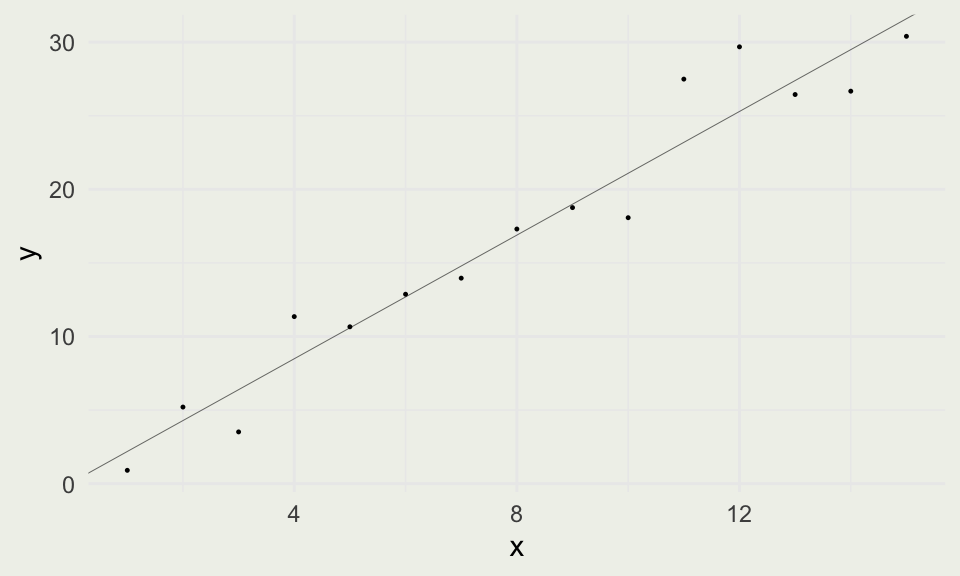
stan_glm
 family:       gaussian [identity]
 formula:      y ~ x
 observations: 15
 predictors:   2
------
            Median MAD_SD
(Intercept) 0.1    1.4
x           2.1    0.2

Auxiliary parameter(s):
      Median MAD_SD
sigma 2.6    0.5

------
* For help interpreting the printed output see ?print.stanreg
* For info on the priors used see ?prior_summary.stanregSMaC: Statistics, Math, and Computing
APSTA-GE 2006: Applied Statistics for Social Science Research
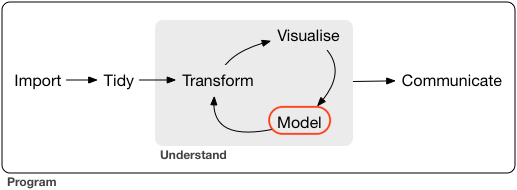
Analysis Workflow
- Following is a high-level, end-to-end view from “R for Data Science” by Wickham and Grolemund
Bayes vs Frequentist Inference
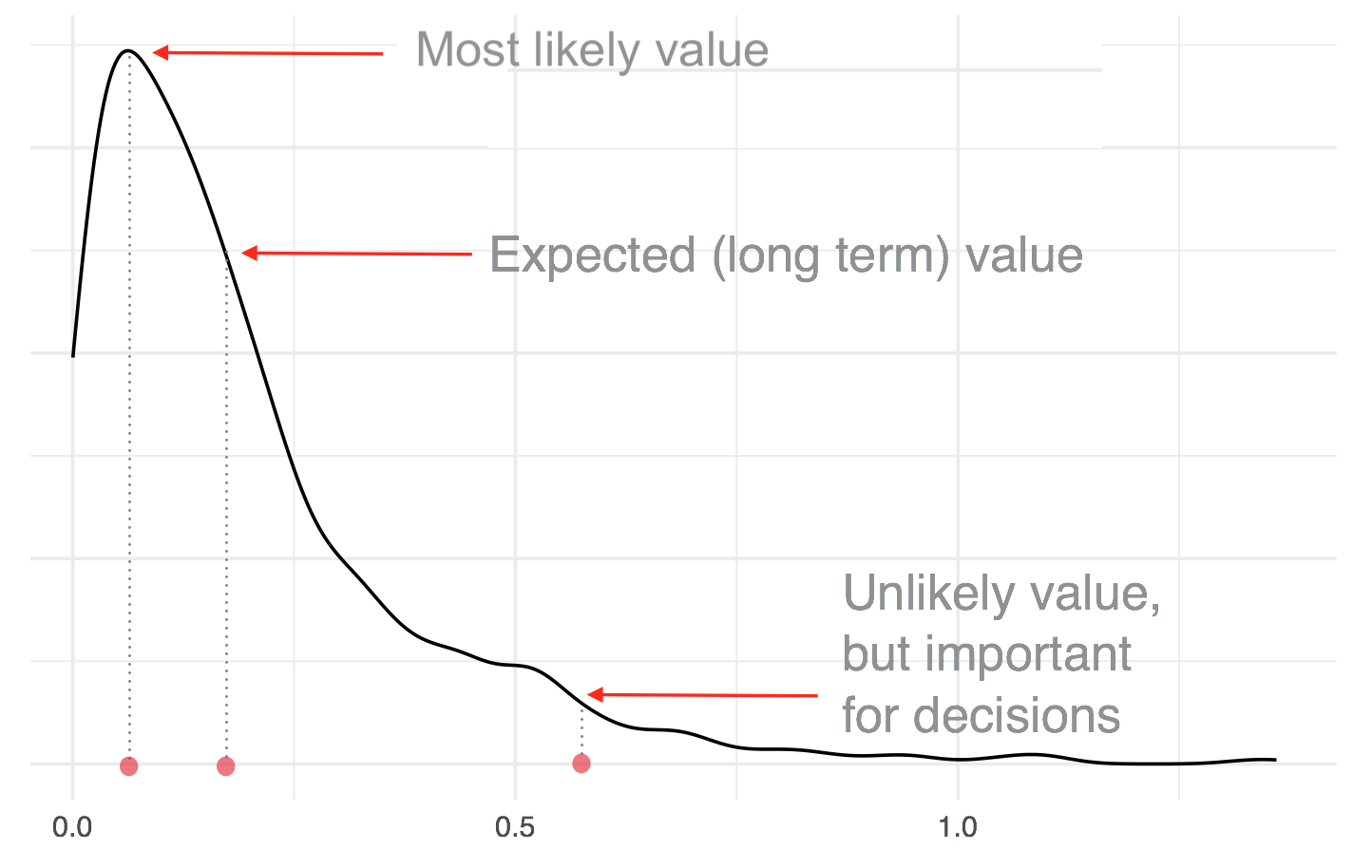
- Estimation is the process of figuring out the unknowns, i.e., unobserved quantities
- In frequentist inference, the problem is framed in terms of the most likely value(s) of \(\theta\)
- Bayesians want to characterize the whole distribution, a much more ambitious goal
- Suppose we want to characterize the following function, which represents some distribution of the unknown parameter:
Simulating a Simple Regression
- We extract our betas using the
coef()R function
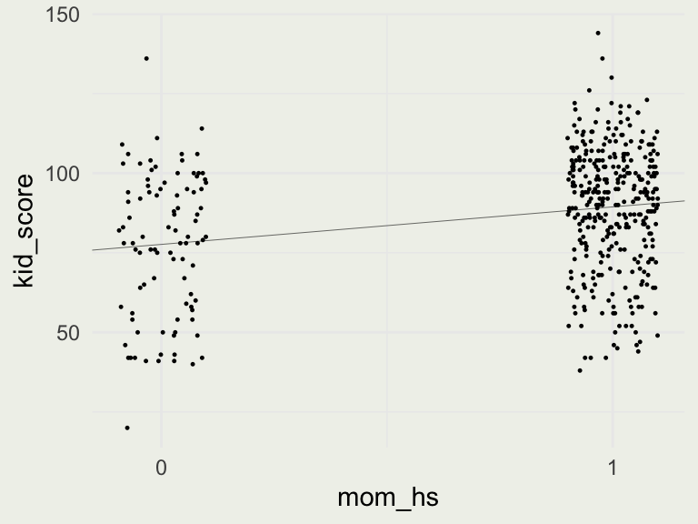
Single Binary Predictor
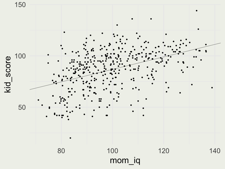
Single Continous Predictor
Visualizing the Fit With Two Predictors
p <- ggplot(aes(mom_iq, kid_score), data = kidiq)
p + geom_point(aes(color = as.factor(mom_hs)), size = 0.2) +
  labs(color = "Mom HS") +
  geom_abline(intercept = coef(fit6)[1], slope = coef(fit6)[3], linewidth = 0.1, color = 'red') +
  geom_abline(intercept = coef(fit6)[1] + coef(fit6)[2], slope = coef(fit6)[3], linewidth = 0.1, color = 'blue')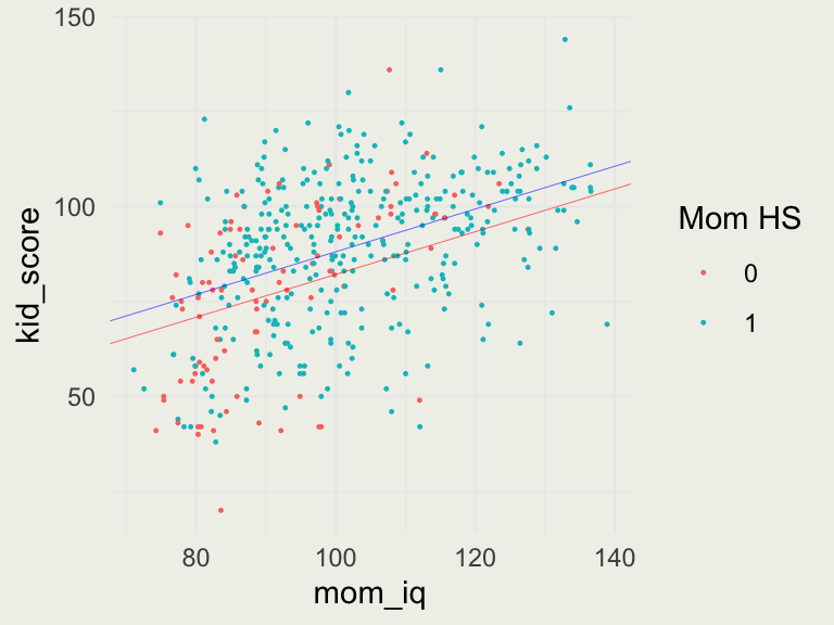
Visualizing Interactions
p <- ggplot(aes(mom_iq, kid_score), data = kidiq)
p + geom_point(aes(color = as.factor(mom_hs)), size = 0.2) +
  labs(color = "Mom HS") +
  geom_abline(intercept = coef(fit7)[1], slope = coef(fit7)[3], linewidth = 0.1, color = 'red') +
  geom_abline(intercept = coef(fit7)[1] + coef(fit7)[2], slope = coef(fit7)[3] + coef(fit7)[4], linewidth = 0.1, color = 'blue')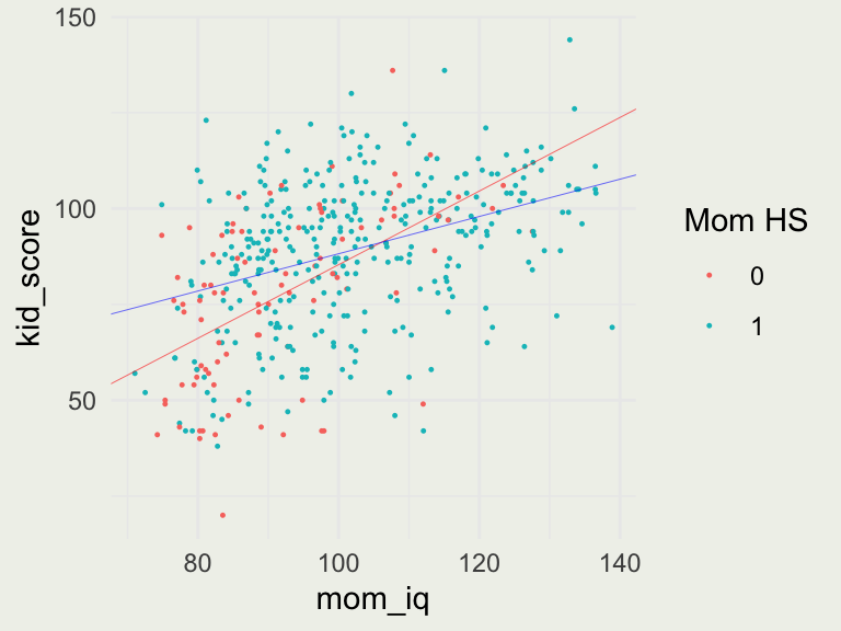
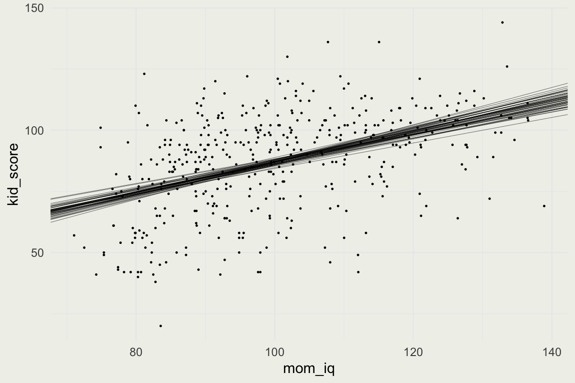
Uncertainty and Prediction
- Using these simulations we display 50 plausible regression lines
Prediction in RStanArm
- We observe a new kid whose mom’s IQ = 120
- Point prediction is shown in Red, 90% uncertainty around the average kid score in Blue, and 90% predictive uncertainty for a new kid is in Yellow.
      1
98.9816 5% 95%
96.5370 101.4359 5% 95%
68.88551 128.75195 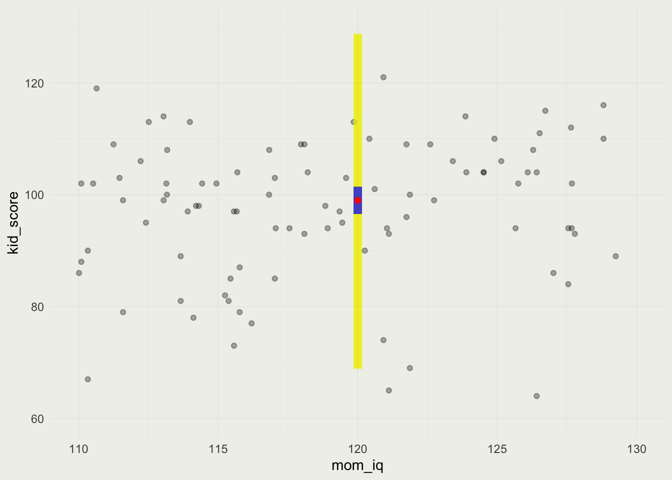
Thanks for being part of my class!

- Lectures: https://ericnovik.github.io/smac.html
- Keep in touch:
- eric.novik@nyu.edu
- https://www.linkedin.com/in/enovik/
- Twitter: @ericnovik
- Personal blog: https://ericnovik.com/