Bayesian Inference

NYU Applied Statistics for Social Science Research
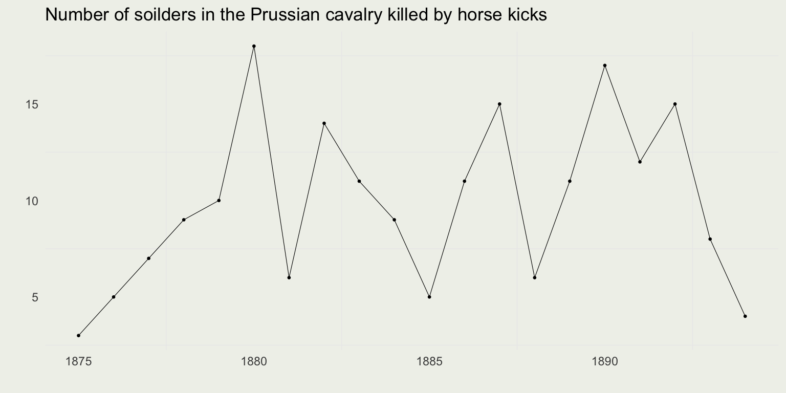
Eric Novik

New York University

Conjugate Models and Posterior Sampling

  • Gamma-Poisson family
  • Normal-Normal family
  • Introduction to posterior sampling on a grid
  • Introduction to Stan
  • Basic Markov Chain diagnostics
  • Effective sample size
  • Computing the R-Hat statistic

\[ \DeclareMathOperator{\E}{\mathbb{E}} \DeclareMathOperator{\P}{\mathbb{P}} \DeclareMathOperator{\V}{\mathbb{V}} \DeclareMathOperator{\L}{\mathcal{L}} \DeclareMathOperator{\I}{\text{I}} \DeclareMathOperator*{\argmax}{arg\,max} \DeclareMathOperator*{\argmin}{arg\,min} \]

Poisson

  • Poisson distribution arises when we are interested in counts

  • In practice, we rarely use Poisson due to its restrictive nature

  • Poisson RV \(Y\) is paremeterized with a rate of occurance \(\lambda\): \(Y|\lambda \sim \text{Pois}(\lambda)\)
    \[ f(y \mid \lambda) = \frac{e^{-\lambda} \lambda^y}{y!}\;\; \text{ for } y \in \{0,1,2,\ldots\} \]

  • Notice, the Tailor series for \(e^\lambda = \sum_{y=0}^{\infty} \frac{\lambda^y}{y!}\) immediately validates that \(f\) is a PDF

  • Also, \(\E(Y | \lambda) = \V(Y | \lambda) = \lambda\), which is the restrictive case mentioned about — real count data seldom satisfied this constraint

Visualizing Poission

  • Notice that as the rate increases, so does the expected number of events as well as variance, which immediately follows from \(\E(Y) = \V(Y) = \lambda\)

Example: Hourse Kicks

  • Serving in Prussian cavalry in the 1800s was a perilous affair
  • Aside from the usual dangers of military service, you were at risk of being killed by a horse kick
  • Data from the book The Law of Small Numbers by Ladislaus Bortkiewicz (1898)
  • Bortkiewicz was a Russian economist and statistician of Polish ancestry
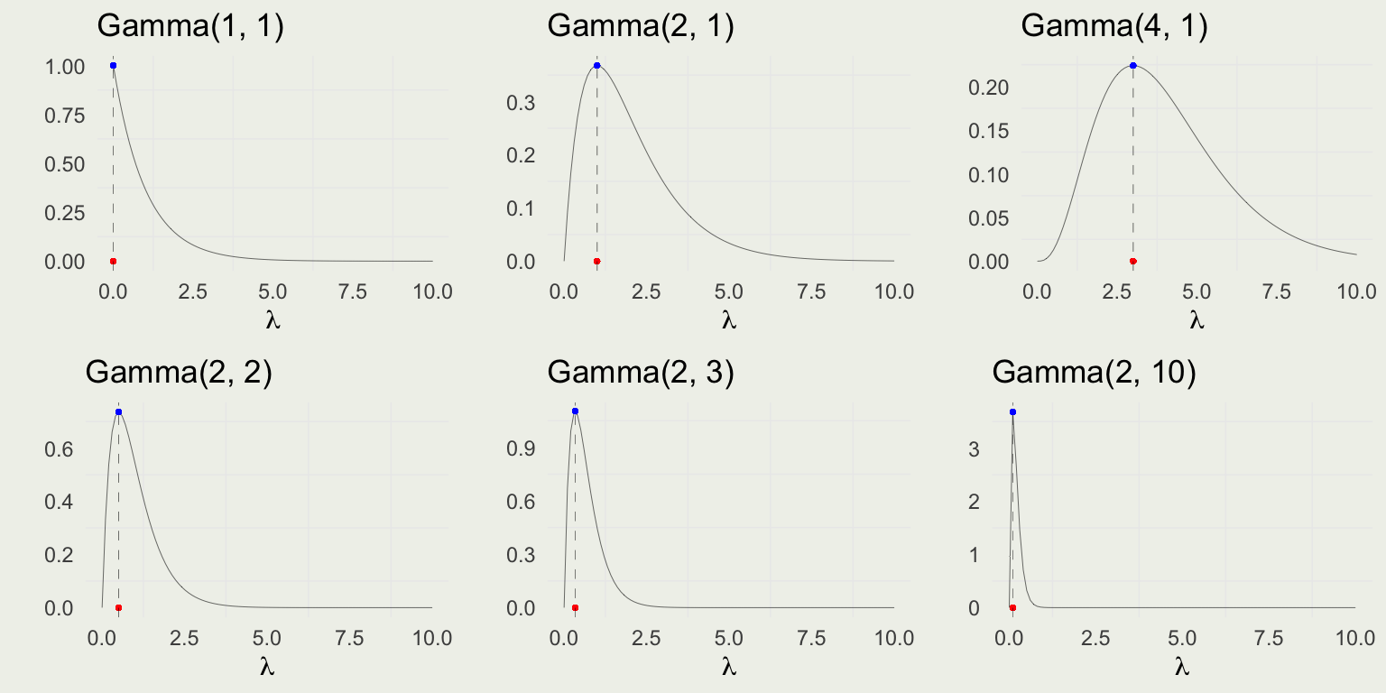
Poisson Likelihood

  • Assume we observe \(Y_1, Y_2, ..., Y_n\) independant Poisson random variables

  • The joint lilelihood, a function of the parameter \(\lambda\) for \(y_i \in \mathbb{Z}^+\) and \(\lambda > 0\), is given by: \[ \begin{eqnarray} f(y \mid \lambda) & = & \prod_{i=1}^n f(y_i \mid \lambda) = f(y_1 \mid \lambda) f(y_2 \mid \lambda) \cdots f(y_n \mid \lambda) = \prod_{i=1}^{n}\frac{\lambda^{y_i}e^{-\lambda}}{y_i!} \\ & = &\frac{\lambda^{y_1}e^{-\lambda}}{y_1!} \cdot \frac{\lambda^{y_2}e^{-\lambda}}{y_2!} \cdots \frac{\lambda^{y_n}e^{-\lambda}}{y_n!} \\ & = &\frac{\left(\lambda^{y_1}\lambda^{y_2} \cdots \lambda^{y_n}\right) \left(e^{-\lambda}e^{-\lambda} \cdots e^{-\lambda}\right)}{y_1! y_2! \cdots y_n!} \\ & = &\frac{\lambda^{\sum_{i=1}^{n} y_i}e^{-n\lambda}}{\prod_{i=1}^n y_i!} \propto \lambda^{\sum_{i=1}^{n} y_i}e^{-n\lambda} \end{eqnarray} \]

  • We call \(\sum_{i=1}^{n} y_i\) a sufficient statistic

Conjugate Prior for Poisson

  • The likelihood has a form of \(\lambda^{a} e^{-b\lambda}\) so we expect the conjugate prior to be of the same form

  • Gamma PDF satisfied this condition: \(f(\lambda) \propto \lambda^{\alpha - 1} e^{-\beta\lambda}\)

  • Matching up the exponents, we can interpret \((\alpha - 1)\) as the total number of incidents \(\sum y_i\) out of \(\beta\) prior observations

  • Full Gamma density is \(\text{Gamma}(\lambda|\alpha,\beta)=\frac{\beta^{\alpha}} {\Gamma(\alpha)} \, \lambda^{\alpha - 1}e^{-\beta \, \lambda}\) for \(\lambda, \alpha, \beta \in \mathbb{R}^+\) \[ \begin{equation} \begin{split} \E(\lambda) & = \frac{\alpha}{\beta} \\ \text{Mode}(\lambda) & = \frac{\alpha - 1}{\beta} \;\; \text{ for } \alpha \ge 1 \\ \V(\lambda) & = \frac{\alpha}{\beta^2} \\ \end{split} \end{equation} \]

  • When \(\alpha = 1\), \(\lambda \sim \text{Dist}(\beta)\). What is \(\text{Dist}\)? Work in pairs.

Visualizing Gamma

  • Notice that variance, mean, and mode are increasing with \(\alpha\)

Gamma Posterior

  • Prior is \(f(\lambda) \propto \lambda^{\alpha - 1} e^{-\beta\lambda}\)

  • Likelihood is \(f(y | \lambda) \propto \lambda^{\sum_{i=1}^{n} y_i}e^{-n\lambda}\) \[ \begin{eqnarray} f(\lambda \mid y) & \propto & \text{prior} \cdot \text{likelihood} \\ & = & \lambda^{\alpha - 1} e^{-\beta\lambda} \cdot \lambda^{\sum_{i=1}^{n} y_i}e^{-n\lambda} \\ & = & \lambda^{\alpha + \sum_{i=1}^{n} y_i - 1} \cdot e^{-\beta\lambda - n\lambda} \\ & = & \lambda^{\color{red}{\alpha + \sum_{i=1}^{n} y_i} - 1} \cdot e^{-\color{red}{(\beta + n)} \lambda} \\ f(\lambda \mid y) & = & \text{Gamma}\left( \alpha + \sum_{i=1}^{n} y_i, \, \beta + n \right) \end{eqnarray} \]

  • As before, we can match the Gamma kernel without doing the integration

Checking the Constant

  • Gamma prior integration constant: \(\frac{\beta^{\alpha}}{\Gamma(\alpha)}\)
  • The posterior kernel integration constant is the reciprocal of: \(\frac{\Gamma(\alpha + \sum y_i)}{(\beta + n)^{\alpha + \sum y_i}}\). Why?
  • We can sanity check this in SymPy, by integrating \(\lambda^{\color{red}{\alpha + \sum_{i=1}^{n} y_i} - 1} \cdot e^{-\color{red}{(\beta + n)} \lambda}\), and letting \(t = \sum y_i\)
import sympy as sp
a, b = sp.symbols('a b', positive=True)
t, n = sp.symbols('t n', positive=True, integer=True)
λ    = sp.symbols('λ', nonnegative=True)
expr = λ**(t + a - 1) * sp.exp(-(n + b) * λ)
result = sp.simplify(sp.integrate(expr, (λ, 0, sp.oo)))

\[\left(b + n\right)^{- a - t} \Gamma\left(a + t\right)\]

Posterior Mean and Variance

Posterior mean and variance follow from the updated prior mean and variance:

\[ \begin{eqnarray} \E(\lambda \mid y) &=& \frac{\alpha'}{\beta'} = \frac{\alpha + \sum_{i=1}^{n} y_i}{\beta + n} \\ \V(\lambda \mid y) &=& \frac{\alpha'}{(\beta')^2} = \frac{\alpha + \sum_{i=1}^{n} y_i}{(\beta + n)^2} \end{eqnarray} \]

Prussian Army Hourse Kicks

  • From 1875 to 1894, there were 14 different cavalry corps
  • Each reported a number of deaths by horse kick every year
  • There are 20 years x 14 corps making 280 observations
library(gt)
d <- vroom::vroom("data/horsekicks.csv")
d |> filter(Year < 1883) |> gt()
Year GC C1 C2 C3 C4 C5 C6 C7 C8 C9 C10 C11 C14 C15
1875 0 0 0 0 0 0 0 1 1 0 0 0 1 0
1876 2 0 0 0 1 0 0 0 0 0 0 0 1 1
1877 2 0 0 0 0 0 1 1 0 0 1 0 2 0
1878 1 2 2 1 1 0 0 0 0 0 1 0 1 0
1879 0 0 0 1 1 2 2 0 1 0 0 2 1 0
1880 0 3 2 1 1 1 0 0 0 2 1 4 3 0
1881 1 0 0 2 1 0 0 1 0 1 0 0 0 0
1882 1 2 0 0 0 0 1 0 1 1 2 1 4 1

Prussian Army Hourse Kicks

# this flattens the data frame into a vector
dd <- unlist(d[, -1]) 
p <- ggplot(aes(y), data = data.frame(y = dd))
p1 <- p + geom_histogram() +
  xlab("Number of deaths reported") + ylab("") +
  ggtitle("Total reported counts of deaths")
p2 <- p + geom_histogram(aes(y = ..count../sum(..count..))) +
  xlab("Number of deaths reported") + ylab("") +
  ggtitle("Proportion of reported counts of deaths")
grid.arrange(p1, p2, nrow = 1)
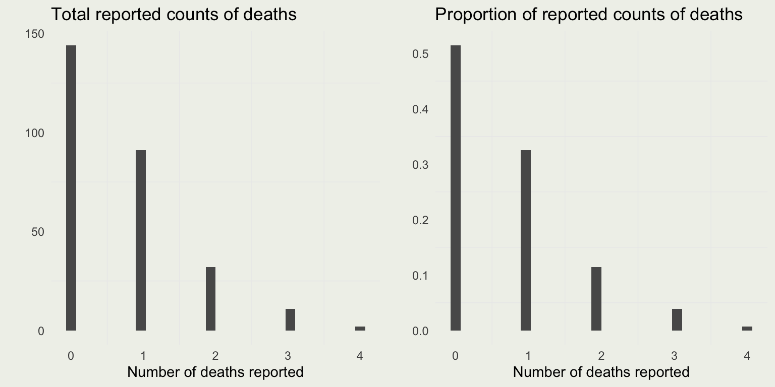
Prussian Army Hourse Kicks

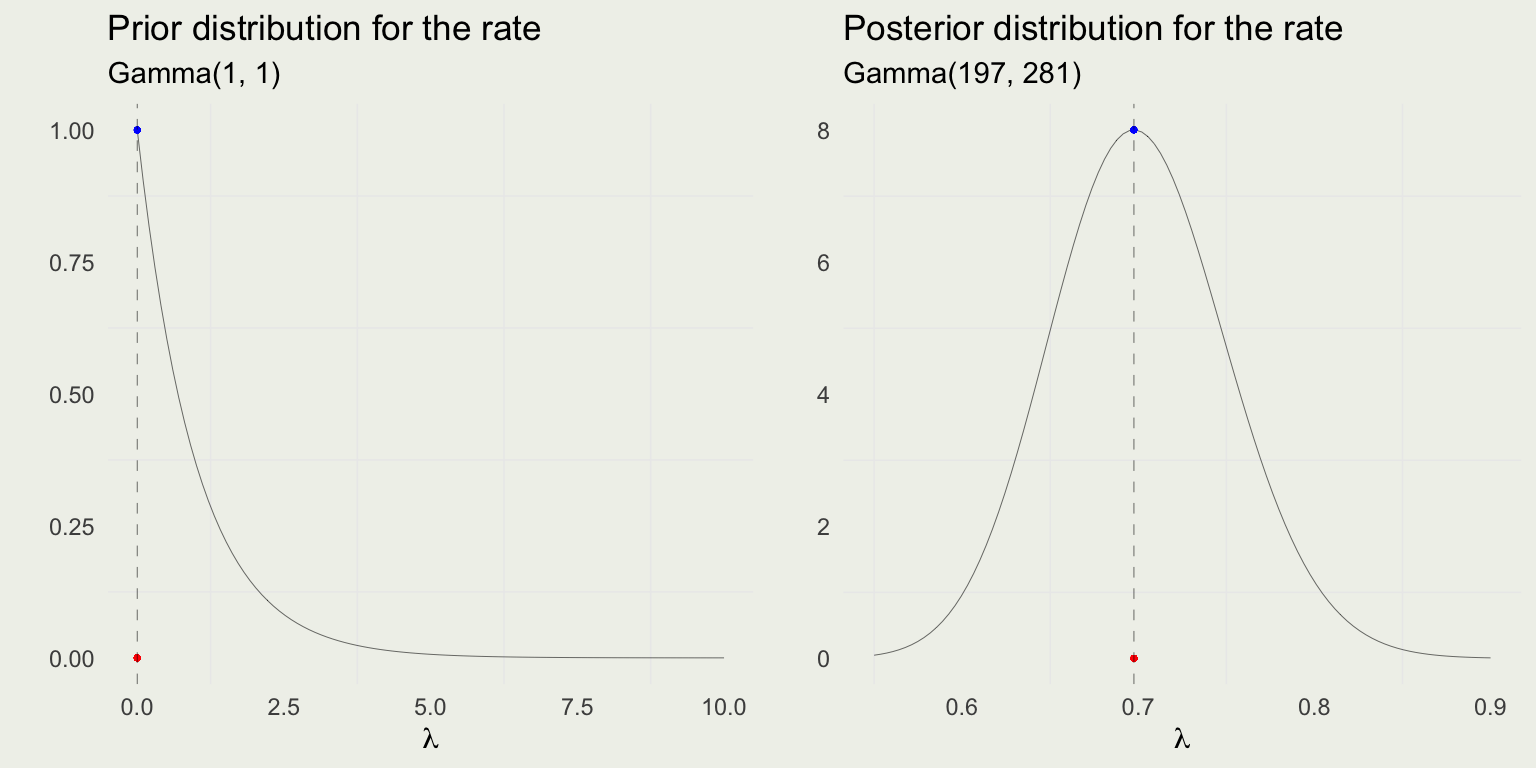
  • Let’s assume that before seeing the data, your friend told you that last year, in 1874, there were no deaths reported in his corps
  • That would imply \(\beta = 1\) and \(\alpha - 1 = 0\) or \(\alpha = 1\)
  • The prior on lambda would therefore be \(\text{Gamma}(1, 1)\)
N <- length(dd)
sum_yi <- sum(dd)
y_bar <- sum_yi/N
cat("Total number of observations N =", N)
Total number of observations N = 280
cat("Total number of deaths =", sum_yi)
Total number of deaths = 196
cat("Average number of deaths =", y_bar)
Average number of deaths = 0.7
  • The posterior is \(\text{Gamma}\left( \alpha + \sum y_i, \, \beta + N \right) = \text{Gamma}(197, \, 281)\)

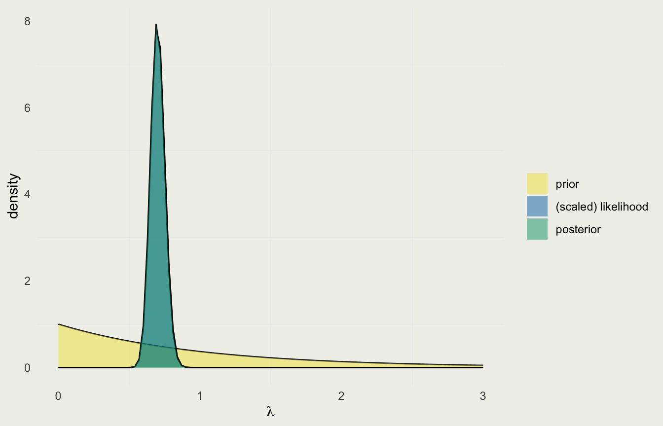
Likelihood Dominates

  • With so much data relative to prior observations, the likelihood completely dominates the prior
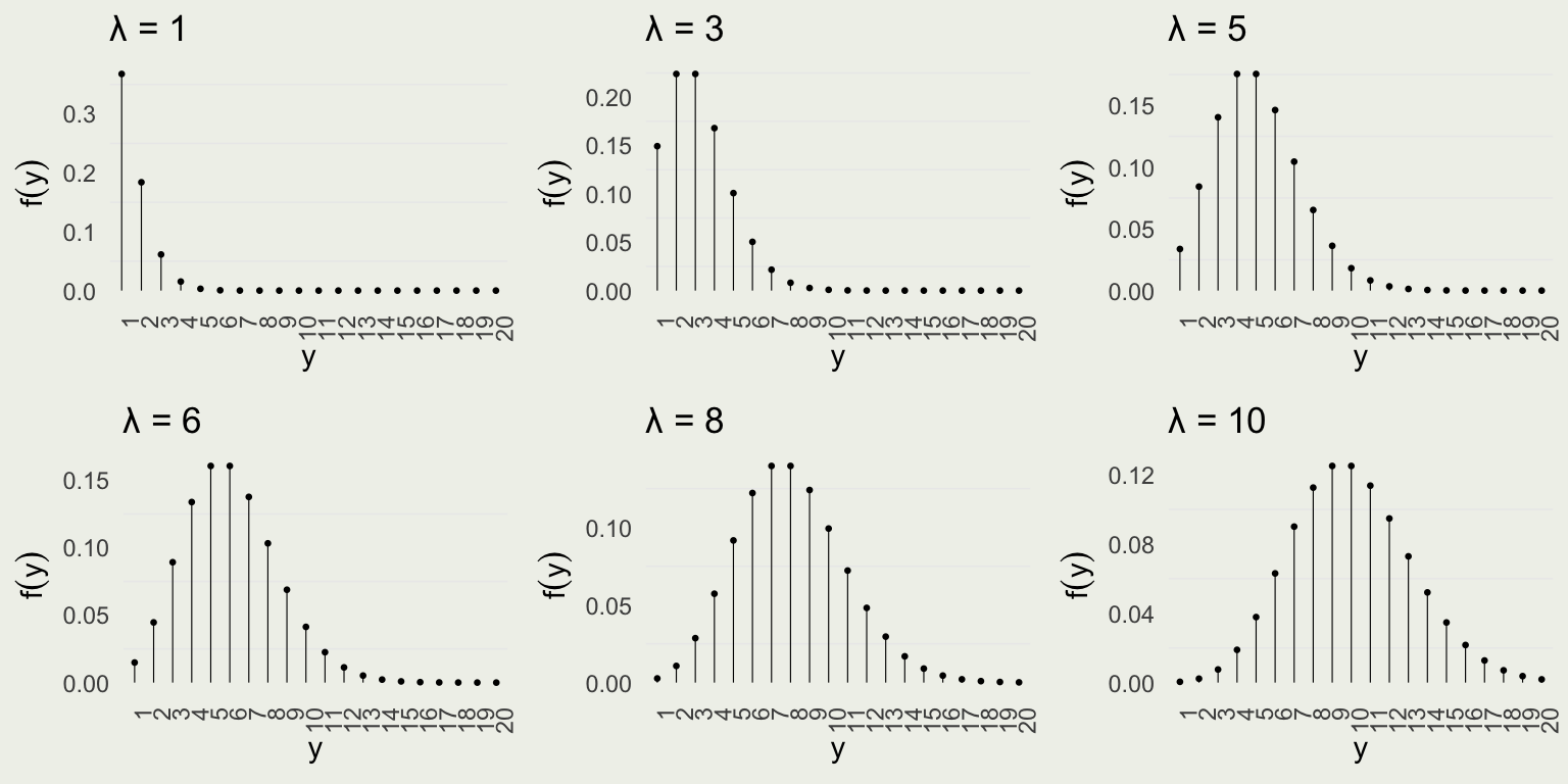
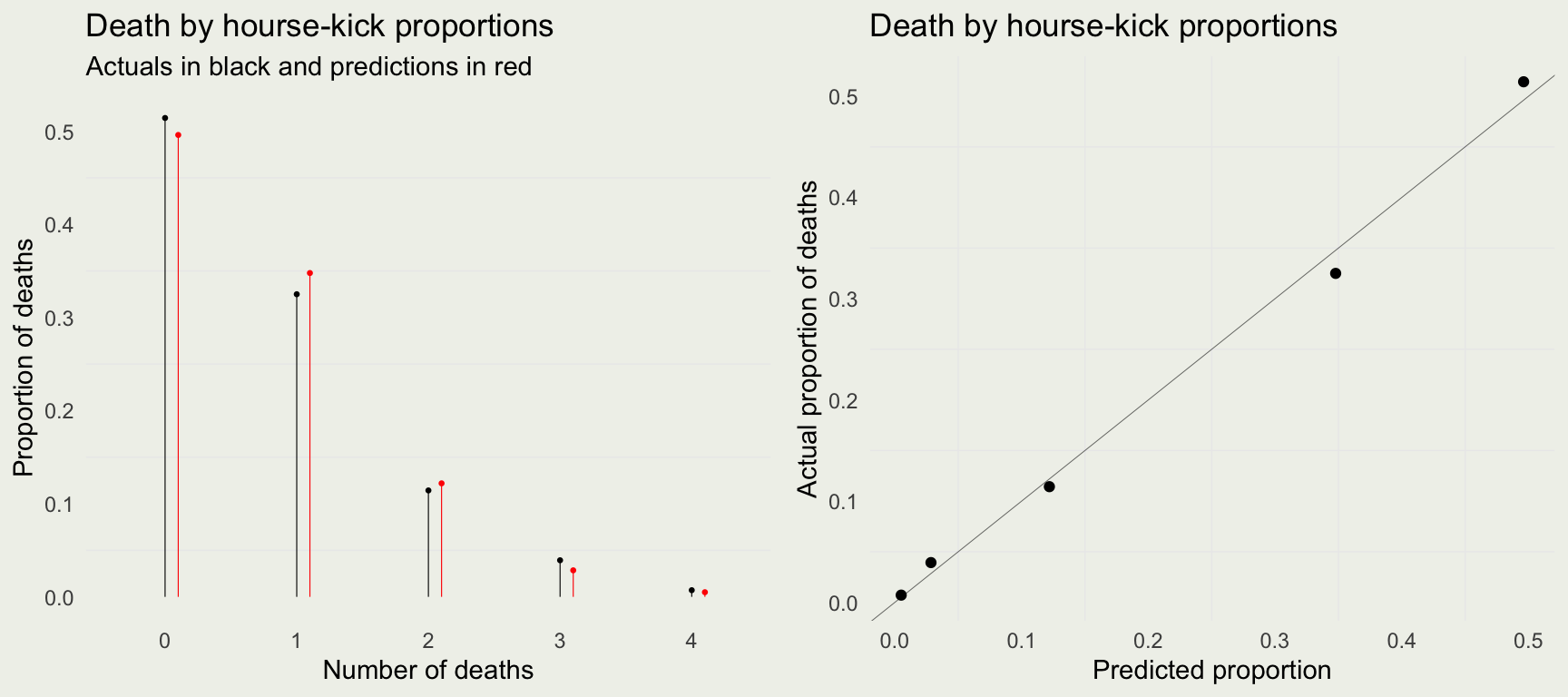
plot_gamma_poisson(1, 1, sum_y = sum_yi, n = N) + 
  xlim(0, 3)

mean_post <- (1 + sum_yi) / (1 + N) 
sd_post <- sqrt((1 + sum_yi) / (1 + N)^2) 
cat("Posterior mean =", mean_post |> round(3))
Posterior mean = 0.701
cat("Average rate =", y_bar)
Average rate = 0.7
cat("Posterior sd =", sd_post |> round(3))
Posterior sd = 0.05

Checking the Fit

  • We can plug the posterior mean for \(\lambda\) into the Poisson PMF
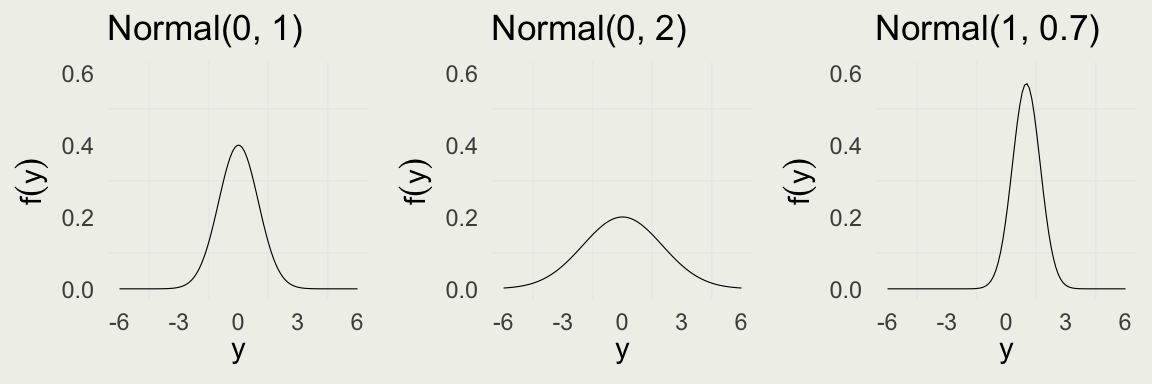
mean_post <- (1 + sum_yi) / (1 + N)
deaths <- 0:4
pred <- dpois(deaths, lambda = mean_post)
actual <- as.numeric(table(dd) / N)

Adding Exposure

  • Poisson likelihood seems to work well for these data
  • It is likely that each of the 16 corps had about the same number of soldier-horses, a common military practice
  • Suppose each corps has a different number of cavalrymen
  • We need to introduce an exposure variable \(x_i\) for each corps unit \[ \begin{eqnarray} y_i & \sim & \text{Poisson}(x_i \lambda)\\ \lambda & \sim & \text{Gamma}(\alpha, \beta) \\ f(y \mid \lambda) & \propto & \lambda^{\sum_{i=1}^{n} y_i}e^{- (\sum_{i=1}^{n} x_i) \lambda} \\ f(\lambda \mid y) & = & \text{Gamma} \left( \alpha + \sum_{i=1}^{n} y_i, \, \beta + \sum_{i=1}^{n} x_i \right) \end{eqnarray} \]

Normal PDF

  • The last conjugate distribution we will introduce is Normal
  • We will only consider a somewhat unrealistic case of known variance \(\sigma \in \mathbb{R}^+\) and unknown mean \(\mu \in \mathbb{R}\)
  • Normal PDF is for one observation \(y\) is given by: \[ \begin{eqnarray} \text{Normal}(y \mid \mu,\sigma) & = &\frac{1}{\sqrt{2 \pi} \ \sigma} \exp\left( - \, \frac{1}{2} \left( \frac{y - \mu}{\sigma} \right)^2 \right) \\ \E(Y) & = & \text{ Mode}(Y) = \mu \\ \V(Y) & = & \sigma^2 \\ \end{eqnarray} \]

Normal PDF

  • Normal arises when many independent small contributions are added up
  • It is a limiting distribution of means of an arbitrary distribution
plot_xbar <- function(n_repl, n_samples) {
  x <- seq(0.6, 1.4, len = 100)
  xbar <- replicate(n_repl, 
                    mean(rexp(n_samples, rate = 1)))
  mu <- dnorm(x, mean = 1, sd = 1/sqrt(n_samples))
  p <- ggplot(aes(x = xbar), 
              data = tibble(xbar))
  p + geom_histogram(aes(y = ..density..), 
                     bins = 30, alpha = 0.6) +
    geom_line(aes(x = x, y = mu), 
              color = 'red', 
              linewidth = 0.3, 
              data = tibble(x, y)) +
    ylab("") + theme(axis.text.y = element_blank())
}

p1 <- plot_xbar(1e4, 100) + 
  ggtitle("Sampling means from rexp(100, 1)")
p2 <- plot_xbar(1e4, 300) + 
  ggtitle("Sampling means from rexp(300, 1)")
grid.arrange(p1, p2, nrow = 2)

Joint Normal Likelihood

  • After observing data \(y\), we can compute the joint normal likelihood, assuming \(\sigma\) is known \[ \begin{eqnarray} f(y \mid \mu) & = & \prod_{i=1}^{n}\frac{1}{\sqrt{2 \pi} \ \sigma} \exp\left( - \, \frac{1}{2} \left( \frac{y_i - \mu}{\sigma} \right)^2 \right) \\ & \propto & \prod_{i=1}^{n} \exp\left( - \, \frac{1}{2} \left( \frac{y_i - \mu}{\sigma} \right)^2 \right) \\ & = & \exp \left( {-\frac{\sum_{i=1}^n(y_i-\mu)^2}{2\sigma^2}}\right) \\ &\propto& \exp\left({-\frac{(\bar{y}-\mu)^2}{2\sigma^2/n}}\right) \end{eqnarray} \]

  • The last line is derived by expanding the square and dropping terms that don’t depend on \(\mu\); \(\bar{y} = \frac{1}{n} \sum_{i=1}^{n} y_i\)

  • Expansion: \(\sum_{i=1}^n (y_i - \mu)^2 = \sum_{i=1}^n \left[(y_i - \bar{y}) + (\bar{y} - \mu)\right]^2\)

Normal Prior

  • We can now define the prior on \(\mu\)
  • We will choose \(\mu\) to be normal: \(\mu \sim \text{Normal}(\theta, \tau^2)\) \[ \begin{eqnarray} f(\mu \mid \theta, \tau) & \propto & \exp\left( - \, \frac{1}{2} \left( \frac{\mu - \theta}{\tau} \right)^2 \right) \\ \end{eqnarray} \]

Normal Posterior

  • For one observation \(y\):

\[ \begin{eqnarray} f(y \mid \mu) & \propto & \exp\left( - \, \frac{1}{2} \left( \frac{y - \mu}{\sigma} \right)^2 \right) \\ f(\mu) & \propto & \exp\left( - \, \frac{1}{2} \left( \frac{\mu - \theta}{\tau} \right)^2 \right) \\ f(\mu \mid y) & \propto & \exp\left( - \, \frac{1}{2} \left( \frac{\mu - \theta}{\tau} \right)^2 - \frac{1}{2} \left( \frac{y - \mu}{\sigma} \right)^2 \right) \\ & = & \exp \left( -\frac{1}{2} \left( \frac{(\mu - \theta)^2}{\tau^2} + \frac{(y - \mu)^2}{\sigma^2} \right)\right) \\ & = & \exp \left( -\frac{1}{2\tau_1^2} \left( \mu - \mu_1 \right)^2 \right) \end{eqnarray} \]

Normal Posterior

  • For one observation: \[ \begin{eqnarray} f(\mu \mid y) &\propto& \exp \left( -\frac{1}{2\tau_1^2} \left( \mu - \mu_1 \right)^2 \right) \text{ i.e. } \mu \mid y \sim \text{Normal}(\mu_1, \tau_1) \\ \mu_1 &=& \frac{\frac{1}{\tau^2} \theta + \frac{1}{\sigma^2} y}{\frac{1}{\tau^2} + \frac{1}{\sigma^2}} \\ \frac{1}{\tau_1^2} &=& \frac{1}{\tau^2} + \frac{1}{\sigma^2} \end{eqnarray} \]

  • For multiple observations: \[ \mu_1 = \frac{\frac{1}{\tau^2} \theta + \frac{n}{\sigma^2} \overline{y}}{\frac{1}{\tau^2} + \frac{n}{\sigma^2}} \\ \frac{1}{\tau_1^2} = \frac{1}{\tau^2} + \frac{n}{\sigma^2} \]

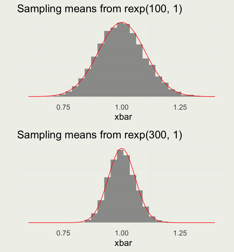
Posterior Simulation

Grid approximation

  • Most posterior distributions do not have an analytical form
  • In those cases, we must resort to sampling methods
  • Sampling in high dimensions requires specialized algorithms
  • Here, we will look at one-dimensional sampling on a grid (of parameter values)
  • At the end of this lecture, we look at some output of a state-of-the-art HMC NUTS sampler
  • Next week, we will examine the Metropolis-Hastings-Rosenbluth algorithm

An example of Gibbs sampling of a Bivariate Normal by Aki Vehtari and Markus Paasiniemi.

Grid approximation

  • We already saw how given samples from the target distribution, we could compute quantities of interest
  • The grid approach to getting samples:
    1. Generate discreet points in parameter space \(\theta\)
    2. Define our likelihood function \(f(y|\theta)\) and prior \(f(\theta)\)
    3. For each point on the grid, compute the product \(f(y|\theta)f(\theta)\)
    4. Normalize the product to sum to 1
    5. Sample from the resulting distribution in proportion to the posterior probability
  • Here, \(\theta\) is continuous, so we can not use the technique we used for a discrete, one-dimensional prior from the clinical trial example.
  • What are some limitations of this approach?

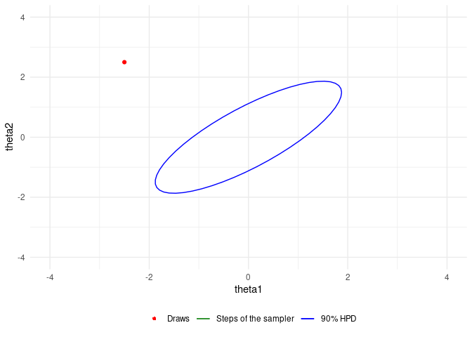
Back to the Binomial

  • For simplicity we will assume uniform \(\text{Beta}(1, 1)\) prior \[ \begin{eqnarray} f(\theta)f(y\mid \theta) &\propto& \theta^{a -1}(1 - \theta)^{b-1} \cdot \prod_{i=1}^{n} \theta^{y_i} (1 - \theta)^{1 - y_i} \\ &=& \theta^0(1 - \theta)^0 \cdot \prod_{i=1}^{n} \theta^{y_i} (1 - \theta)^{1 - y_i} \\ &=& \prod_{i=1}^{n} \theta^{y_i} (1 - \theta)^{1 - y_i} \\ &=& \theta^{\sum_{i=1}^{n} y_i} \cdot (1 - \theta)^{\sum_{i=1}^{n} (1- y_i)} \end{eqnarray} \]
  • On the log scale: \(\log f(\theta, y) \propto \log(\theta) \cdot\sum_{i=1}^{n} y_i + \log(1 - \theta) \cdot\sum_{i=1}^{n} (1-y_i)\)
  • Suppose that 3 out of 5 patients responded to treatment
  • Model: \(\text{lp}(\theta) = \log(\theta) \cdot\sum_{i=1}^{n} y_i + \log(1 - \theta) \cdot\sum_{i=1}^{n} (1-y_i)\)
lp <- function(theta, data) {
# log(theta) * sum(data$y) + log(1 - theta) * sum(1 - data$y)
  lp <- 0
  for (i in 1:data$N) {
    lp <- lp + log(theta) * data$y[i] + log(1 - theta) * (1 - data$y[i])
  }
  return(lp)
}
data <- list(N = 5, y = c(0, 1, 1, 0, 1))
# generate theta parameter grid
theta <- seq(0.01, 0.99, len = 100)
# compute log likelihood and prior for every value of the grid
log_lik <- lp(theta, data); log_prior <- log(dbeta(theta, 1, 1))
# compute log posterior
log_post <- log_lik + log_prior
# convert back to the original scale and normalize
post <- exp(log_post); post <- post / sum(post)
# sample theta in proportion to the posterior probability
draws <- sample(theta, size = 1e5, replace = TRUE, prob = post)
  • From the first lecture, we know the posterior is \(\text{Beta}(1 + 3, 1 + 5 - 3) = \text{Beta}(4, 3)\)
  • We can compare this density to the posterior draws
beta_dens <- dbeta(theta, 4, 3)
(mle <- sum(data$y) / data$N)
[1] 0.6

Monte Carlo Integration and MCMC

  • We already saw a special case of MC integration

  • Suppose we can draw samples from PDF \(f\), \((\theta^{(1)}, \theta^{(2)},..., \theta^{(N)})\)

  • If we want to compute an expectation of some function \(h\): \[ \begin{eqnarray} \E_f[h(\theta)] &=& \int h(\theta)f(\theta)\, d\theta &\approx& \frac{1}{N} \sum_{i = 1}^{N} h \left( \theta^{(i)} \right) \end{eqnarray} \]

  • The Law of Large Numbers tells us that these approximations improve with \(N\)

  • In practice, the challenge is obtaining draws from \(f\)

  • That’s where MCMC comes in

  • Suppose we want to estimate the mean and variance of standard normal
  • In case of the mean, \(h(\theta) := \theta\) and variance, \(h(\theta) := \theta^2\), and \(f(\theta) = \frac{1}{\sqrt{2 \pi} \ } e^{-\theta^2/2}\) \[ \begin{eqnarray} \E[\theta] &=& \int_{-\infty}^{\infty} \theta f(\theta)\, d\theta &\approx& \frac{1}{N} \sum_{i = 1}^{N} \theta^{(i)} \\ \E[\theta^2] &=& \int_{-\infty}^{\infty} \theta^2 f(\theta)\, d\theta &\approx& \frac{1}{N} \sum_{i = 1}^{N} \left( \theta^{(i)} \right)^2 \end{eqnarray} \]
N <- 1e5
theta <- rnorm(N, 0, 1)          # draw theta from N(0, 1)
(1/N * sum(theta)) |> round(2)   # E(theta),   same as mean(theta)
[1] 0
(1/N * sum(theta^2)) |> round(2) # E(theta^2), same as mean(theta^2)
[1] 1
  • Suppose we want to estimate a CDF of Normal(0, 1) at some point \(t\)
  • We let \(h(\theta) = \I(\theta < t)\), where \(\I\) is an indicator function that returns 1 when \(\theta < t\) and \(0\) otherwise \[ \begin{eqnarray} \E[h(\theta)] = \E[\I(\theta < t)] &=& \int_{-\infty}^{\infty} \I(\theta < t) f(\theta)\, d\theta = \int_{-\infty}^{t}f(\theta)\, d\theta = \Phi(t) \\ &\approx& \frac{1}{N} \sum_{i = 1}^{N} \I(\theta^{(i)} < t) \\ \end{eqnarray} \]
pnorm(1, 0, 1) |> round(2)          # Evalute N(0, 1) CDF at 1
[1] 0.84
N <- 1e5
theta <- rnorm(N, 0, 1)             # draw theta from N(0, 1)
(1/N * sum(theta < 1)) |> round(2)  # same as mean(theta < 1)
[1] 0.84
  • MCMC is a very general method for computing expectations (integrals)
  • It produces dependant (autocorrelated) samples, but for a good algorithm, the dependence is manageable
  • Stan’s MCMC algorithm is very efficient (more on that later) and requires all parameters to be continuous (data can be discrete)
  • It solves the problem of drawing from distribution \(f(\theta)\) where \(f\) is not one of the fundamental distributions and \(\theta\) is high dimentional
  • What is high-dimensional? Modern algorithms like NUTS can jointly sample tens of thousands and more parameters
  • That’s 10,000+ dimensional integrals of complicated functions!

Introduction to Stan

  • Stan is a procedural, statically typed, Turning complete, probabilistic programming language
  • Stan language expresses a probabilistic model
  • Stan transpiler converts it to C++
  • Stan inference algorithms perform parameter estimation
  • Our model: \(\text{lp}(\theta) = \log(\theta) \cdot\sum_{i=1}^{n} y_i + \log(1 - \theta) \cdot\sum_{i=1}^{n} (1-y_i)\)
// 01-bernoulli.stan
data {
  int<lower=0> N;
  array[N] int<lower=0, upper=1> y;
}
parameters {
  real<lower=0, upper=1> theta;
}
model {
  for (i in 1:N) {
    target += log(theta * y[i] + 
              log(1 - theta) * (1 - y[i]);
  }
}
// 02-bernoulli.stan
data {
  int<lower=0> N;
  array[N] int<lower=0, upper=1> y;
}
parameters {
  real<lower=0, upper=1> theta;
}
model {
  theta ~ beta(1, 1);
  y ~ bernoulli(theta);
}

Running Stan

library(cmdstanr)

m1 <- cmdstan_model("stan/01-bernoulli.stan") # compile the model
data <- list(N = 5, y = c(0, 1, 1, 0, 1))
f1 <- m1$sample(       # for other options to sample, help(sample)
  data = data,         # pass data as a list, match the vars name to Stan
  seed = 123,          # to reproduce results, Stan does not rely on R's seed
  chains = 4,          # total chains, the more, the better
  parallel_chains = 4, # for multi-processor CPUs
  refresh = 0,         # number of iterations printed on the screen
  iter_warmup = 500,   # number of draws for warmup (per chain)
  iter_sampling = 500  # number of draws for samples (per chain)
)
Running MCMC with 4 parallel chains...

Chain 1 finished in 0.0 seconds.
Chain 2 finished in 0.0 seconds.
Chain 3 finished in 0.0 seconds.
Chain 4 finished in 0.0 seconds.

All 4 chains finished successfully.
Mean chain execution time: 0.0 seconds.
Total execution time: 0.3 seconds.
f1$summary()
# A tibble: 2 × 10
  variable   mean median    sd   mad     q5    q95  rhat ess_bulk ess_tail
  <chr>     <dbl>  <dbl> <dbl> <dbl>  <dbl>  <dbl> <dbl>    <dbl>    <dbl>
1 lp__     -5.30  -5.02  0.734 0.320 -6.82  -4.78   1.00     800.    1024.
2 theta     0.566  0.577 0.173 0.187  0.273  0.833  1.01     860.     986.

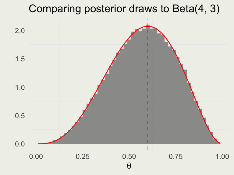
Working With Posterior Draws

library(tidybayes)

draws <- gather_draws(f1, theta, lp__)
tail(draws) # draws is a tidy long format
# A tibble: 6 × 5
# Groups:   .variable [1]
  .chain .iteration .draw .variable .value
   <int>      <int> <int> <chr>      <dbl>
1      4        495  1995 lp__       -4.84
2      4        496  1996 lp__       -4.85
3      4        497  1997 lp__       -4.83
4      4        498  1998 lp__       -5.04
5      4        499  1999 lp__       -4.78
6      4        500  2000 lp__       -4.78
draws |> 
  group_by(.variable) |> 
  summarize(mean = mean(.value))
# A tibble: 2 × 2
  .variable   mean
  <chr>      <dbl>
1 lp__      -5.30 
2 theta      0.566
median_qi(draws, .width = 0.90)
# A tibble: 2 × 7
  .variable .value .lower .upper .width .point .interval
  <chr>      <dbl>  <dbl>  <dbl>  <dbl> <chr>  <chr>    
1 lp__      -5.02  -6.82  -4.78     0.9 median qi       
2 theta      0.577  0.273  0.833    0.9 median qi       
draws <- spread_draws(f1, theta, lp__)
tail(draws) # draws is a tidy wide format
# A tibble: 6 × 5
  .chain .iteration .draw theta  lp__
   <int>      <int> <int> <dbl> <dbl>
1      4        495  1995 0.505 -4.84
2      4        496  1996 0.503 -4.85
3      4        497  1997 0.510 -4.83
4      4        498  1998 0.436 -5.04
5      4        499  1999 0.568 -4.78
6      4        500  2000 0.582 -4.78
theta <- seq(0.01, 0.99, len = 100)
p <- ggplot(aes(theta), data = draws)
p + geom_histogram(aes(y = after_stat(density)), 
                   bins = 30, alpha = 0.6) +
    geom_line(aes(theta, beta_dens), 
              linewidth = 0.5, color = 'red',
              data = tibble(theta, beta_dens)) +
  ylab("") + xlab(expression(theta)) +
  ggtitle("Posterior draws from Stan")
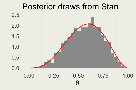
What’s a Chain

A is a sequence of random variables \(\{X_n\}_{n \geq 0}\) defined on a state space \(S\) such that for all \(n \geq 0\) and for any states \(i_0, i_1, \dots, i_{n+1} \in S\), the Markov property holds:

\[ \mathbb{P}(X_{n+1}=j \mid X_0=i_0, X_{n-1}=i_{n-1}, \dots, X_n=i_n) = \mathbb{P}(X_{n+1}=j \mid X_n=i) \]

The transition probabilities are represented by a matrix \(Q\), where:

\[ q_{ij} = \mathbb{P}(X_{n+1} = j \mid X_n = i) \]

Dynamic Simulation

MCMC Demo

MCMC Diagnostics

  • In general, you want to assess (1) the quality of the draws and (2) the quality of predictions
  • There are no guarantees in either case, but the former is easier than the latter
  • The folk theorem of statistical computing: computational problems often point to problems in the model (AG)
  • We will address the quality of the draws now and the quality of predictions later in the course

Example of bad markov chains, page 283, Figure 11.3, BDA 3.

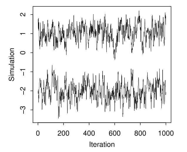
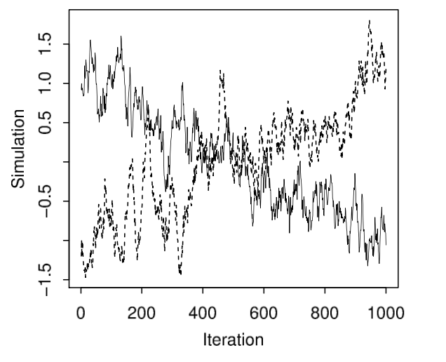
Good Chain Bad Chain

library(bayesplot)
draws <- f1$draws("theta")
color_scheme_set("viridis")
p1 <- mcmc_trace(draws, pars = "theta") + ylab(expression(theta)) +
  ggtitle("Good Chain")
bad_post <- readRDS("data/bad_post.rds")
bad_draws <- bad_post$draws("mu")
p2 <- mcmc_trace(bad_draws, pars = "mu") + ylab(expression(theta)) +
  ggtitle("Bad Chain")
grid.arrange(p1, p2, nrow = 2)

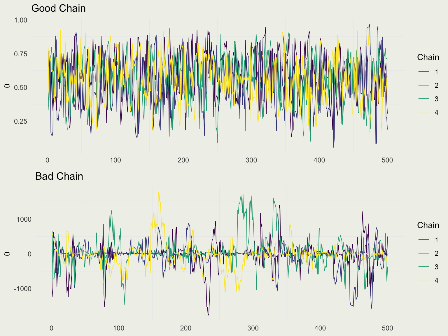
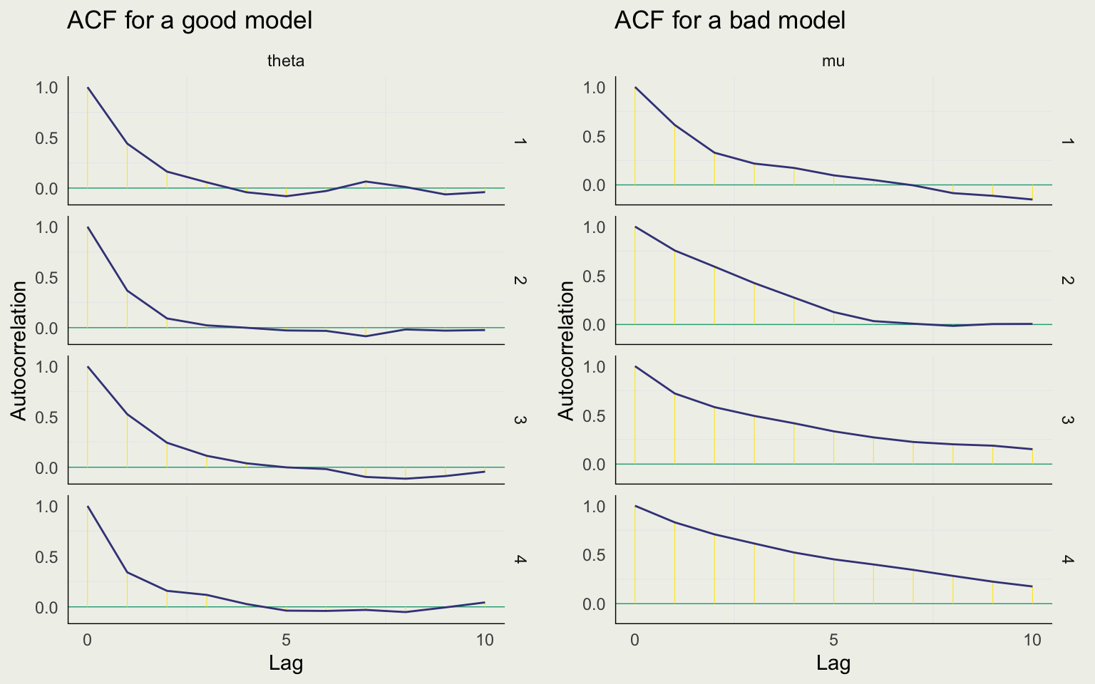
Effective Sample Size and Autocorrelation

  • MCMC generates dependent draws from the target distribution
  • Dependent samples are less efficient as you need more of them to estimate the quantity of interest
  • ESS or \(N_{eff}\) is approximately how many independent samples you have
  • Typically, \(N_{eff} < N\) for MCMC, as there is some autocorrelation
  • ESS should be considered relative to \(N\): \(\frac{N_{eff}}{N}\)
  • Generally, we don’t like to see \(\text{ratio} < 0.10\)
neff_ratio(f1, pars = "theta") |> round(2)
theta 
 0.43 
neff_ratio(bad_post, pars = "mu") |> round(2)
  mu 
0.09 

Computing R-Hat

  • Autocorrelation assesses the quality of a single chain

  • Split R-Hat estimates the extent to which the chains are consistent with one another

  • It does it by assessing the mixing of chains by comparing variances within and between chains (technically sequences, as chains are split up) \[ \begin{eqnarray} \hat{R} = \sqrt{\frac{\frac{n-1}{n}\V_W + \frac{1}{n}\V_B}{\V_W}} = \sqrt{\frac{\V_{\text{total}}}{\V_{W}}} \end{eqnarray} \]

  • \(\V_W\) is within chain variance and \(\V_B\) is between chain variance

  • We don’t like to see R-hats greater than 1.02 and really don’t like them greater than 1.05

bayesplot::rhat(f1, pars = "theta") |> round(3)
theta 
1.006 
bayesplot::rhat(bad_post, pars = "sigma")  |> round(3)
sigma 
1.043 

Stan Homework

  1. Modify the program to incorporate Beta(2, 2) without using theta ~ beta(2, 2) (i.e. using target +=)
  2. Modify the program to account for an arbitrary Beta(a, b) distribution
  3. Verify that you got the right result in #1 by a) comparing Stan’s posterior means and posterior standard deviations to the means and standard deviations under the conjugate model; b) modifying the Stan program using beta(2, 2) prior and Bernoulli likelihood shown here; c) modifying the R code to get a third point of comparison.
  • Hint: For #2, pass parameters a and b in the data block
data {
  int<lower=0> N;
  array[N] int<lower=0, upper=1> y;
}
parameters {
  real<lower=0, upper=1> theta;
}
model {
  for (i in 1:N) {
    target += log(theta * y[i] + 
              log(1 - theta) * (1 - y[i]);
  }
}